Abstract

We discuss the concept of connected, reparameterization invariant matter correlators in quantum gravity. We analyze the effect of discretization in two solvable cases : branched polymers and two-dimensional simplicial gravity. In both cases the naively defined connected correlators for a fixed volume display an anomalous behavior, which could be interpreted as a long-range order. We suggest that this is in fact only a highly non-trivial finite-size effect and propose an improved definition of the connected correlator, which reduces the effect. Using this definition we illustrate the appearance of a long-range spin order in the Ising model on a two-dimensional random lattice in an external magnetic field $H$, when $H\to 0$ and $\beta=\beta_{C}$.

1 Introduction

In a theory where gravity is quantized it is non-trivial to define the concept of a connected correlation function. The problem is only apparent once one has a genuine non-perturbative definition of quantum gravity where one can go beyond the expansion around flat space. To exemplify the problem let us define a reparameterization invariant correlation function in quantum gravity:

$$G^{\phi_{1}\phi_{2}}_{\Lambda}(R)=\int{\cal D}[g]\int{\cal D}[X]\;e^{-S_{\Lambda}}\;\int\int dV_{g}(\xi)\,dV_{g}(\xi^{\prime})\;\phi_{1}(\xi)\phi_{2}(\xi^{\prime})\;\delta(D_{g}(\xi,\xi^{\prime})-R).$$ (1)

Here $dV_{g}$ is the invariant volume element and $D_{g}(\xi,\xi^{\prime})$ the geodesic distance between $\xi$ and $\xi^{\prime}$ for a given metric $g$. ${\cal D}[X]$ symbolizes the integration over additional degrees of freedom of the theory, i.e.  the matter fields and $\phi_{i}$ are local observables built from these fields and/or the gravitational field. The functional integral is over equivalence classes of metrics, i.e. the group of diffeomorphisms is divided out. Finally $\Lambda$ is the cosmological constant, i.e. we have the following decomposition of the action:

$$S_{\Lambda}=\Lambda V_{g}+S_{V}[g,X],~{}~{}~{}~{}~{}V_{g}=\int dV_{g}(\xi),$$ (2)

where $S_{V}$ is independent of the cosmological constant. As we can see from (1) the correlator involves three rather than two non-trivial operators, contrary to the flat space case, where the definition of a distance does not involve an extra operator. The new element is the geometric “separator”, which for any non-trivial geometry becomes a complicated non-local object. A partition function for quantum gravity can be defined by

$$Z_{\Lambda}=\int{\cal D}[g]\int{\cal D}[X]\;e^{-S_{\Lambda}},$$ (3)

and $G^{\phi_{1}\phi_{2}}_{\Lambda}(R)$ is an unnormalized correlation function. The simplest object of this kind is a “geometric” two-point function, including only the “separator”:

$$G^{11}_{\Lambda}(R)=\int{\cal D}[g]\int{\cal D}[X]\;e^{-S_{\Lambda}}\;\int\int dV_{g}(\xi)dV_{g}(\xi^{\prime})\;\delta(D_{g}(\xi,\xi^{\prime})-R),$$ (4)

i.e. the same object as in (1), just with $\phi(\xi)\to 1$. $G^{11}_{\Lambda}(R)$ can be viewed as the partition function for the ensemble of universes where two marked points are separated by a geodesic distance $R$. We have

$$\int_{0}^{\infty}dR\;G^{11}_{\Lambda}(R)=\frac{\partial^{2}}{\partial\Lambda^{2}}Z_{\Lambda}\equiv{\tilde{Z}}_{\Lambda}$$ (5)

This two-point function plays a special role in describing the geometric properties of the system [1]. In general $G^{11}_{\Lambda}(R)$ is expected to fall off exponentially, reflecting the fact that there is an exponentially small probability to create a universe where two points are separated by a geodesic distance $R$ much larger than some power of the cosmological constant. This power sets the geometric scale of the system, or a relation between the average radius $\left\langle R\right\rangle$ and the average volume $\left\langle V\right\rangle$ of the universe: $\left\langle V\right\rangle\propto\left\langle R\right\rangle^{d_{h}}$, where $d_{h}$ is the Hausdorff dimension. The concept of a geometric scale $\left\langle R\right\rangle$ is very important when we discuss the problem of matter correlations, which in principle may involve some other “physical” scale. The geometric scale is controlled by the cosmological constant, while the physical scale will in general depend on some other coupling constants, describing the matter sector of the theory. Away from the critical point in this sector we expect the physical scale to be small compared with the geometric scale. Only then we can expect to distinguish those two scales In the following we shall always assume that it is the case. With a small abuse of notation, we call this limit the thermodynamic limit. Close to the critical point the two scales become comparable and there we may expect to find a non-trivial coupling between the matter and gravitational sectors of the theory. If we view $G^{11}_{\Lambda}(R)$ as a partition function, the distance $R$ plays the role of an additional coupling constant of the theory. All these peculiarities make the definition of connected correlators difficult and sometimes ambiguous.

A priori we have various possibilities of defining a normalized correlation function. Let us mention two different definitions:

$$\left\langle\phi_{1}\phi_{2}\right\rangle_{\Lambda}(R)=\frac{G^{\phi_{1}\phi_{2}}_{\Lambda}(R)}{{\tilde{Z}}_{\Lambda}}$$ (6)

and

$$\left\langle\phi_{1}\phi_{2}\right\rangle_{\Lambda}(R)=\frac{G^{\phi_{1}\phi_{2}}_{\Lambda}(R)}{G^{11}_{\Lambda}(R)}.$$ (7)

The definitions differ by the way geometry is counted. In (7) it is counted in the same way in numerator and denominator. In fact, if $\phi_{1}$ and $\phi_{2}$ are independent observables which do not couple to gravity at all, definition (6) gives

$$\left\langle\phi_{1}\phi_{2}\right\rangle_{\Lambda}(R)=\left\langle\phi_{1}\right\rangle\left\langle\phi_{2}\right\rangle\frac{G^{11}_{\Lambda}(R)}{{\tilde{Z}}_{\Lambda}},$$ (8)

On the other hand, the definition (7) leads to

$$\left\langle\phi_{1}\phi_{2}\right\rangle_{\Lambda}(R)=\left\langle\phi_{1}\right\rangle\left\langle\phi_{2}\right\rangle,$$ (9)

independent of $R$.

The results (8) or (9) are trivial from the point of view of the correlation functions. Both should be viewed as examples of a situation, where the observables $\phi_{i}$ at different points are uncorrelated. The correlator can in this case be expressed as a product of three single-operator averages, which is best seen in (8). One would expect a similar structure of the correlation function in the thermodynamic limit when the observables $\phi_{i}$ do couple to gravity, but when the distance between the two points $R$ is much bigger than the correlation length. The expectation values $\left\langle\phi_{i}\right\rangle$ should then be replaced by $\left\langle\phi_{i}\right\rangle_{\Lambda}$ implying the non-trivial dependence on the cosmological constant. The $R$ dependence should factorize, like in (8) or (9).

At smaller distances there may be deviations from a simple factorization . The obvious questions are: Can these be interpreted as a signal of a correlation between the fields? Which type of behavior can still be attributed to the uncorrelated operators? Such questions clearly can not be answered without some hint from a solvable model. Unfortunately the number of solvable theories, where one can actually compute the two-point functions, is very limited. In the next section we shall present some exact results concerning operators which we believe are uncorrelated.

Of course a behavior like (8) and (9) can not be observed if we have correlators with infinite correlation length (or where the geometric and physical scales become comparable), as will be the case when we consider correlators between the conformal fields coupled to two-dimensional quantum gravity.

To obtain a consistent definition of the matter correlation length we must define the concept of a connected correlation function. Various definitions have been given in the literature [3, 4, 5] and below we summarize the discussion. First we face the problem of a sensible definition of $\left\langle\phi\right\rangle_{\Lambda}$. Several choices seem possible, but in order to match the definitions of correlation functions, as given by (6) or (7) one can use either

$$\left\langle\phi\right\rangle_{\Lambda}=\frac{1}{{\tilde{Z}}_{\Lambda}}\int{\cal D}[g]\int{\cal D}[X]\;e^{-S_{\Lambda}}\;{V_{g}}\int dV_{g}(\xi)\,\phi(\xi)=\frac{\int_{0}^{\infty}dR\;G^{\phi 1}_{\Lambda}(R)}{\int_{0}^{\infty}dR\;G^{11}_{\Lambda}(R)}$$ (10)

or

$$\left\langle\phi\right\rangle_{\Lambda}(R)\equiv\left\langle\phi\,1\right\rangle_{\Lambda}(R)=\frac{G^{\phi\,1}_{\Lambda}(R)}{G^{11}_{\Lambda}(R)}$$ (11)

The last definition depends on the geodesic distance $R$, and it is from this point of view slightly unusual as a definition of an expectation value of a field. But not much more than in usual field theory where the lack of translational invariance caused by an external field can introduce a space-time dependence in $\left\langle\phi\right\rangle$. As discussed above, such dependence is expected to disappear for large $R$ implying the existence of a well defined limit $\left\langle\phi\right\rangle_{\Lambda}(R\to\infty)$. In fact, this limit should agree with the value defined by (10) provided the correlation length of the matter fields is (much) less than the average radius of the universe. The definition of $\left\langle\phi\right\rangle_{\Lambda}$ is related to the correlation between the $\phi$ and unit operators, as is clear from (10) and (11). Thus the statement that the two definitions of $\left\langle\phi\right\rangle$ agree in the thermodynamic limit, for large $R$ is equivalent to the statement that we have a factorization

$$G^{\phi\,1}_{\Lambda}(R)\approx\left\langle\phi\right\rangle_{\Lambda}G^{11}_{\Lambda}(R)$$ (12)

for such values of $R$. In general we would expect the unit operator to be uncorrelated with any other operator, so naively we would expect (12) to be satisfied almost for any value of $R$. This can be checked numerically.

Note that the correlation function $G^{\phi 1}_{\Lambda}(R)$ almost inevitably enters in any sensible definition of the connected part of a correlator since one has to consider an object like

$$\left\langle\phi_{1}\phi_{2}\right\rangle^{con}_{\Lambda}(R)\equiv\left\langle(\phi_{1}-\left\langle\phi_{1}\right\rangle 1)(\phi_{2}-\left\langle\phi_{2}\right\rangle 1)\right\rangle_{\Lambda}(R),$$ (13)

with some definition of $\left\langle\phi_{i}\right\rangle$. If we use (11) as a definition of $\left\langle\phi_{i}\right\rangle$ and (7) as a definition of the correlator, then eq. (13) fulfills the standard decomposition and can be written as

$$\left\langle\phi_{1}\phi_{2}\right\rangle_{\Lambda}(R)-\left\langle\phi\right\rangle_{\Lambda}(R)\left\langle\phi_{2}\right\rangle_{L}(R).$$ (14)

If we use (6) and (10) instead, eq. (13) can be written as

$$\left\langle\phi_{1}\phi_{2}\right\rangle^{con}_{\Lambda}(R)=$$

$$\frac{1}{{\tilde{Z}}_{\Lambda}}\;(G^{\phi_{1}\phi_{2}}_{\Lambda}(R)-\left\langle\phi_{1}\right\rangle_{\Lambda}G^{1\phi_{2}}_{\Lambda}(R)-\left\langle\phi_{2}\right\rangle_{\Lambda}G^{1\phi_{1}}_{\Lambda}(R)+\left\langle\phi_{1}\right\rangle_{\Lambda}\left\langle\phi_{2}\right\rangle_{\Lambda}G^{11}_{\Lambda}(R).$$

In this case one does not have the standard local decomposition as in eq. (14), but integrating over $R$ one obtains:

$$\left\langle\phi_{1}\phi_{2}\right\rangle_{\Lambda}-\left\langle\phi_{1}\right\rangle_{\Lambda}\left\langle\phi_{2}\right\rangle_{\Lambda},$$ (16)

where the first term in (16) is the usual integrated correlator as known from two-dimensional quantum gravity:

$$\left\langle\phi\phi\right\rangle_{\Lambda}=\frac{1}{{\tilde{Z}}_{\Lambda}}\int{\cal D}[g]\int{\cal D}[X]\;e^{-S_{\Lambda}}\;\int\int dV_{g}(\xi)dV_{g}(\xi^{\prime})\;\phi(\xi)\phi(\xi^{\prime}).$$ (17)

We can now define the correlation length by the exponential decay of $\left\langle\phi\phi\right\rangle_{\Lambda}^{con}(R)$, defined either by (14) or (1) and the thermodynamic limit is where this correlation length is much smaller than the average radius of the the universe.

The fixed volume partition functions ${\tilde{Z}}_{V}$ and $G^{\phi_{1}\phi_{2}}_{V}(R)$ are related to ${\tilde{Z}}_{\Lambda}$ and $G^{\phi_{1}\phi_{2}}_{\Lambda}(R)$ by Laplace transformations

$${\tilde{Z}}_{\Lambda}=\int^{\infty}_{0}dV\;e^{-\Lambda V}Z_{V},~{}~{}~{}~{}~{}~{}G^{\phi_{1}\phi_{2}}_{\Lambda}(R)=\int^{\infty}_{0}dV\;G^{\phi_{1}\phi_{2}}_{V}(R).$$ (18)

and it is natural to use the definition of correlators, expectation values of fields and connected correlators corresponding to eqs. (6), (8), (10) and (1), just with the the partition functions for fixed $\Lambda$ replaced by the ones for fixed volume $V$, given by (18). Note in particular that we have

$$\left\langle\phi\right\rangle_{V}=\frac{1}{Z_{V}}\int{\cal D}[g]\,\delta(\int dV_{g}(\xi)\!-\!V)\;\int{\cal D}[X]\;\;e^{-S_{V}[g,X]}\;\frac{1}{V_{g}}\int dV_{g}(\xi)\;\phi(X;\xi),$$ (19)

as one would have expected. The connected correlator for finite volume could thus be defined as

$$\left\langle\phi_{1}\phi_{2}\right\rangle^{con}_{V}(R)=$$

$$\frac{1}{V^{2}Z_{V}}\;\Big{(}G^{\phi_{1}\phi_{2}}_{V}(R)-\left\langle\phi_{1}\right\rangle_{V}G^{1\phi_{2}}_{V}(R)-\left\langle\phi_{2}\right\rangle_{V}G^{1\phi_{1}}_{V}(R)+\left\langle\phi_{1}\right\rangle_{V}\left\langle\phi_{2}\right\rangle_{V}G^{11}_{V}(R)\Big{)},$$

with the normalized fixed volume correlators defined as

$$\bar{G}^{11}_{V}(R)=\frac{1}{V^{2}Z_{V}}G^{11}_{V}(R),$$ (21)

satisfying

$$\int_{0}^{\infty}dR\;\bar{G}^{11}_{V}(R)=V.$$ (22)

As we show in the next Section, the discrete regularization of a theory may, and in fact does lead to some complications, where the finite volume effects tend to mimic the physical correlations even in situations where there are no correlations in the grand canonical formulation. This was first realized in [5].

2 Analytical results

There are unfortunately very few systems, where the concepts presented above can be compared with the analytic prediction. We present here the few models where the two-point function can be explicitly calculated. These systems are branched polymers [6, 7] and two-dimensional simplicial gravity [1, 8, 9]. In both cases one defines a discretized (integer) geodesic distance $r$ between the points of the manifold. The physical relation between the the continuum and discrete geodesic distances is

$$R=ra,$$ (23)

with the lattice spacing $a\to 0$ in the continuum limit, but the distance $R$ kept fixed. In both cases the relation between the the continuum volume $V$ and the discrete volume $N$ is anomalous :

$$V=Na^{d_{h}},$$ (24)

where $d_{h}$ is the Hausdorff dimension of the system, equal 2 for a generic branched polymer and 4 for two-dimensional simplicial gravity.

In both cases there is no extra matter content in the theory and the only observables we can discuss are related to the local geometric properties of the manifold. In the case of simplicial quantum gravity these can be some functions of the coordination number of a vertex, in the case of branched polymers – functions of the branching ratio at a vertex. Both cases correspond to the observables, which we expect to be essentially uncorrelated for $r>0$.

2.1 Branched polymers

Let us start by repeating the discussion of the simpler case of the branched polymers [6, 7]. The partition function in this model is given as a weighted sum over the ensemble of trees. Trees are weighted by one-vertex branching weights $p(q_{i})$. The partition function for the ensemble of trees is given by :

$$\bar{Z}=\sum_{N}\exp(-\mu N)\;\sum_{T\in{\mathcal{T}}_{N}}\frac{1}{C(T)}\prod_{i\in T}p(q_{i})$$ (25)

where $q_{i}$ is the order of a vertex $i$, $N$ is the number of vertices and $C(T)$ is an appropriate symmetry factor of the graph; $\mu$ plays the role of the bare cosmological constant.

The correlation functions are constructed by means of the partition function $Z$ of planted, rooted, planar trees. This partition function can be found from the following recursive equation [6]:

$$Z=e^{-\mu}F(Z)$$ (26)

where

$$F(Z)=\sum_{q=1}p(q)Z^{q-1}\,.$$ (27)

In the generic case equation (26) has a critical point $\mu_{C}$ for which

$$e^{-\mu_{C}}F^{\prime}(Z_{0})=1,~{}~{}~{}~{}~{}Z_{0}=Z(\mu_{C}).$$

For $\mu$ approaching the critical value $\mu_{C}$ from above, $Z$ has the following singularity :

$$Z(\mu)=Z_{0}-Z^{\prime}_{1}\sqrt{\mu-\mu_{c}}+{\cal O}(\mu-\mu_{c})$$ (28)

The natural definition of a distance $r$ between two vertices of a graph is the number of links joining these vertices. The discrete analogue of the geometric two-point function can be calculated in terms of $Z(\mu)$ [5, 6, 7] as

$$G_{\mu}^{11}(r)=\Big{(}1+\frac{Z}{\partial_{\mu}Z}\Big{)}^{r-1}Z^{2}.$$ (29)

The factor $Z^{2}$ in (29) is a contribution from the two ends of the chain. Close to the critical point

$$\Delta=-\log(1+\frac{Z}{\partial_{\mu}Z})\propto\sqrt{\mu-\mu_{c}}+{\cal O}(\mu-\mu_{c}).$$ (30)

and (29) becomes

$$G_{\mu}^{11}(r)=\exp(-(r-1)\Delta)Z(\Delta)^{2}.$$ (31)

In a branched polymer system the only local observables we can construct are functions of vertex orders $q_{1},q_{2}$ at the end points. Replacing $Z\to Z~{}e^{\lambda_{i}}F(Ze^{\lambda_{i}})/F(Z)$ at the end points we obtain a generating function of all such observables: differentiating with respect to $\lambda_{i}$ at $\lambda_{i}=0$ we generate powers of $q_{i}$, $i=1,2$. Notice that for $Z$ satisfying (26) the generating function

$${\cal G}(\lambda)=\frac{e^{\lambda}F(Ze^{\lambda})}{F(Z)}=\sum_{n}\left\langle q^{n}\right\rangle_{\mu}\frac{\lambda^{n}}{n!}=\left\langle\hat{{\cal G}}(\lambda)\right\rangle_{\mu},$$ (32)

where the averages are taken with respect to the partition function $Z(\mu)$. We conclude that for every choice of observables we have a simple factorization

$$G_{\mu}^{\{\lambda_{1},\lambda_{2}\}}(r)={\cal G}(\lambda_{1}){\cal G}(\lambda_{2})G_{\mu}^{11}(r),$$ (33)

which proves a lack of correlation between any pair of vertex order operators at points $1$ and $2$.

Near the critical point the generating function ${\cal G}(\lambda)$ can be expanded as

$${\cal G}(\lambda)={\cal G}_{0}(\lambda)+\Delta{\cal G}_{1}(\lambda)+{\cal O}(\Delta^{2})$$ (34)

Using the simple form (31) of $G_{\mu}^{11}(r)$ we get

$$G_{\mu}^{\{\lambda_{1},\lambda_{2}\}}(r) = \Big{(}{\cal G}_{0}(\lambda_{1})+{\cal G}_{1}(\lambda_{1})\partial_{r}+\cdots\Big{)}\Big{(}{\cal G}_{0}(\lambda_{2})+{\cal G}_{1}(\lambda_{2})\partial_{r}+\cdots\Big{)}G_{\mu}^{11}(r)$$ (35)

$$\approx {\cal G}_{0}(\lambda_{1}){\cal G}_{0}(\lambda_{2})G_{\mu}^{11}(r+\delta(\lambda_{1})+\delta(\lambda_{2})),$$

where we have introduced a shift

$$\delta(\lambda)=\frac{{\cal G}_{1}(\lambda)}{{\cal G}_{0}(\lambda)},$$ (36)

and where the dots stand for higher order terms typically proportional to $d^{2}G_{\mu}^{11}(r)/dr^{2}$.

2.2 2d gravity

Two-dimensional simplicial gravity can be obtained as the planar limit of the $\phi^{3}$ matrix theory. The coupling constant $g=e^{-\mu}$ of this theory can be parametrized as

$$8g^{2}=s(1-s^{2}).$$ (37)

In this parameterization $g=0$ corresponds to $s=1$ and the critical value $g^{2}_{c}=1/12\sqrt{3}$. In the planar limit each $\phi^{3}$ vertex is dual to a triangle and a $\phi^{3}$ graph can be viewed as a two-dimensional surface built from triangles, expansion in powers of $g$ becoming the expansion in the area of the surface. Following [9] we construct the transfer matrix [10]

$$G_{\mu}(X,Y;r)=\sum_{L,L^{\prime}}X^{L}Y^{L^{\prime}}G_{\mu}(L,L^{\prime};r),$$ (38)

where $G_{\mu}(L,L^{\prime};r)$ is the sum of all possible connected planar $\phi^{3}$ graphs with boundaries being the loops (planarly ordered sequences of external links) with lengths $L$ and $L^{\prime}$, separated by a “distance” $r$. The distance between the two vertices of a graph is the length of the shortest path following the links of a graph. The transfer matrix $G_{\mu}(X,Y;r)$ can be calculated using the “peeling” method [11] giving

$$G_{\mu}(X,Y;r)=\frac{f_{\mu}(\hat{X})}{f_{\mu}(X)}\frac{1}{1-\hat{X}Y},$$ (39)

where

$$f_{\mu}(X,g)=(1-\frac{sX}{g})\sqrt{1-\frac{4gX}{s^{2}}}$$ (40)

and $\hat{X}(X,r)$ satisfies

$$r = -\frac{1}{\Delta}\log\frac{T(\hat{X})}{T(X)},$$ (41)

$$\Delta = s\sqrt{1-\frac{4g^{2}}{s^{3}}}.$$

$$T(X) = \frac{1-\frac{\Delta}{\sqrt{s^{2}-4gX}}}{1+\frac{\Delta}{\sqrt{s^{2}-4gX}}}.$$

For $g\to g_{c}=e^{-\mu_{c}}$ we have

$$\mu-\mu_{c}\propto\Delta^{4}+\cdots$$

which reflects the fact that the Hausdorff dimension $d_{h}=4$. Introducing $\hat{T}=T(\hat{X})$ and $T(X)=e^{-\Delta r_{0}(X)}$ we have

$$\hat{T}=e^{-\Delta(r+r_{0}(X))}.$$ (42)

Using this parameterization we easily express $f_{\mu}(\hat{X},g)$ as

$$f_{\mu}(\hat{X},g) = \frac{\Delta^{3}}{g^{2}}\coth({1\over 2}\Delta(r+r_{0}))(1-\coth^{2}({1\over 2}\Delta(r+r_{0})))$$

$$= F(\Delta(r+r_{0})).$$

The transfer matrix described above can be used to calculate the two-point correlators [1, 2]. Below we shall discuss only the simpler case, when one of the operators is the unit operator. The solution for the general case with two non-trivial operators can be deduced from symmetry. The first step will be to close the incoming loop. We are still left with the open final loop. The resulting function will be denoted by $\bar{G}_{\mu}(X;r)$ and can be expressed as

$$\bar{G}_{\mu}(X;r) = \oint_{C_{Y}}\frac{dY}{2\pi{\rm i}Y}G_{\mu}(X,\frac{1}{Y};r)Y\frac{\partial}{\partial Y}\Psi(Y)$$ (44)

$$= \frac{f_{\mu}(\hat{X})}{f_{\mu}(X)}\hat{X}\frac{\partial}{\partial\hat{X}}\Psi(\hat{X}),$$ (45)

where

$$\Psi(X)=\frac{1}{2}(\frac{X}{g}+1)+\frac{1}{2}(1-\frac{sX}{g})\sqrt{1-\frac{4gX}{s^{2}}}$$ (46)

is a generating function of the connected Green’s functions of the $\phi^{3}$ matrix model [16]. For small $\Delta$ the effect of closing the incoming loop can be represented as

$$\bar{G}_{\mu}(X;r) = \frac{F(\Delta(r+r_{0}))-\partial_{r}F(\Delta(r+r_{0}))+\cdots}{F(\Delta r_{0})}$$

$$\approx \frac{F(\Delta(r-1+r_{0}))}{F(\Delta r_{0})}.$$

The dots correspond to terms proportional to the second derivative of $F$. The $X$ dependence in this formula appears through $r_{0}=r_{0}(X)$. This is exactly the information we need. The particular choice of a set of operators we wish to study is not very important, provided the incoming lines represented by the $X$ dependence are attached to some local geometric object. The simplest choice is just a line, joining the end points, which leads to the generating function

$$G_{\mu}^{\{\lambda_{1},\lambda_{2}=0\}}(r)=\bar{G}_{\mu}(X=g~{}e^{\lambda_{1}};r),$$ (48)

where we introduced, as before, the parameter $\lambda_{1}$ to count the length of the line and its higher moments. Notice that although the $r$ dependence of this quantity is more complicated than in the branched polymer case, the fundamental properties remain the same. Denoting by $\delta(\lambda)=r_{0}(\lambda)-r_{0}(0)$ we have

$$G_{\mu}^{\{\lambda_{1},\lambda_{2}=0\}}(r)={\cal G}(\lambda_{1})G_{\mu}^{11}(r+\delta(\lambda_{1})).$$ (49)

where

$${\cal G}(\lambda)=\frac{F(\Delta r_{0}(0))}{F(\Delta r_{0}(\lambda))}.$$

Again the correlation function involving the nontrivial operator ($\lambda\neq 0$) is related to that of the unit operator ($\lambda=0$) by a $\lambda$-dependent multiplicative factor and a $\lambda$-dependent shift of $r$.

2.3 The Ansatz for a connected correlator

There are two important lessons one can learn from the examples presented above. The first one is that even in cases where there is no correlation the naive factorization of the two-point correlator:

$$G_{\mu}^{1\phi}(r)=\left\langle\phi\right\rangle_{\mu}G_{\mu}^{11}(r)$$ (50)

is satisfied only asymptotically, for large enough $r$. This does not necessarily mean that there is no simple factorization, as we see from the example of pure 2d gravity, (see (42)). The object for which we observe a simple behavior is not the two-point function itself, but rather a geometric object, natural to the evolution of the characteristic equation of the transfer matrix. The two-point function is itself expressible in terms of this object. Near the critical point the geometric scale of the system is provided by $\Delta$ and the relation between the cosmological constant and this parameter is anomalous

$$\mu-\mu_{c}\propto\Delta^{d_{h}}.$$

In general only for $r$ large enough the correlation function $G_{\mu}^{11}(r)$ has a simple exponential form.

The second lesson is that we can nevertheless extend the idea of factorization to be satisfied for the whole range of $r$ if instead of (50) we use the modified Ansatz:

$$G_{\mu}^{1\phi}(r)=(A_{\phi}-B_{\phi}~{}\partial_{r}+\cdots)G_{\mu}^{11}(r)$$ (51)

which asymptotically (for $r$ large enough for $G_{\mu}^{11}(r)$ to be purely exponential) corresponds to

$$\left\langle\phi\right\rangle_{\mu}=A_{\phi}+B_{\phi}~{}\Delta+\cdots$$

To order ${\cal O}(\Delta)$ the Ansatz (51) can be viewed as an additional shift:

$$G_{\mu}^{1\phi}(r)=A_{\phi}~{}G_{\mu}^{11}(r+\delta_{\phi})$$ (52)

with

$$\delta_{\phi}=\frac{B_{\phi}}{A_{\phi}}.$$

For two uncorrelated operators the corresponding Ansatz would be

$$G_{\mu}^{\phi_{1}\phi_{2}}(r)=A_{\phi_{1}}~{}A_{\phi_{2}}~{}G_{\mu}^{11}(r+\delta_{1}+\delta_{2})+{\cal O}(\Delta^{2}).$$ (53)

The additional shifts are specific for the operator and are additive. We also made an assumption that $A_{\phi_{i}}\neq 0$. The uncorrelated contribution described above has to be subtracted if one is interested in the connected correlation function. The effect described above is a finite-size correction. In the continuum limit $r\to R/a$ and $\partial_{r}\to a~{}\partial_{R}$. It is however very important if we analyze the system using the fixed volume canonical numerical simulations.

The unnormalized correlation function $G_{\mu}^{\phi_{1}\phi_{2}}(r)$ can be represented as a (discrete) Laplace transform of the fixed-$N$ contributions as

$$G_{\mu}^{\phi_{1}\phi_{2}}(r)=\sum_{N}\exp(-\mu N)\;C_{N}~{}G_{N}^{\phi_{1}\phi_{2}}(r),$$ (54)

where $C_{N}$ controls the normalization of the fixed-volume correlation function and is independent of $\phi$. The commonly used normalization corresponds to

$$\sum_{r}~{}G_{N}^{11}(r)=N.$$ (55)

Using standard arguments $G_{N}^{\phi_{1}\phi_{2}}(r)$ can be obtained by inverting the Laplace transform (54). From (35) it follows that

$$G_{N}^{\phi_{1}\phi_{2}}(r)=\Big{(}A_{\phi_{1}}-B_{\phi_{1}}\partial_{r}+\cdots\Big{)}\Big{(}A_{\phi_{2}}-B_{\phi_{2}}\partial_{r}+\cdots\Big{)}G_{N}^{11}(r)\approx A_{\phi_{1}}~{}A_{\phi_{2}}~{}G_{N}^{11}(r+\delta_{1}+\delta_{2}).$$ (56)

In the large-$N$ limit we expect

$$G_{N}^{11}(r)\approx N^{1-1/d_{h}}g(x),$$ (57)

where the scaling variable $x=(r+\delta_{0})/N^{1/d_{h}}$. It is clear from (56) that derivatives $\partial_{r}$ produce finite-size corrections ${\cal O}(1/N^{1/d_{h}})$ or ${\cal O}(1/L)$, where $L$ is the linear (discrete) size of the system.

In a numerical experiment at a fixed volume $N$ one measures the correlation functions $G_{N}^{11}(r)$, $G_{N}^{1\phi_{i}}(r)$ and $G_{N}^{\phi_{1}\phi_{2}}(r)$, where $G_{N}^{11}(r)$ is normalized as in (55). As we argued above we expect to ${\cal O}(1/L^{2})$

$$G_{N}^{1\phi_{i}}(r)=A_{\phi_{i}}G_{N}^{11}(r+\delta_{i}).$$ (58)

This behavior can easily be checked in numerical experiments and we find it satisfied with amazing accuracy, not only in cases discussed above, but also for other two-dimensional systems, as will be discussed in the next section as well as in correlation experiments in four-dimensional simplicial gravity [17]. Following (58) one would expect $A_{i}$ to be an $N$-independent constant $A_{\phi_{i}}=\left\langle\phi_{i}\right\rangle_{N=\infty}$. Experimentally we found that an excellent fit to (58) corresponds to the choice $A_{\phi_{i}}=\left\langle\phi_{i}\right\rangle_{N}$, which for an extensive quantity differs by ${\cal O}(1/N)$.

In general the corrrelation function $G_{N}^{\phi_{1}\phi_{2}}(r)$ may contain the non-trivial connected part. However if we define the connected part of the correlator in the analogy with (1) as

$$G_{N}^{\phi_{1}\phi_{2},conn}(r)=$$

$$G^{\phi_{1}\phi_{2}}_{N}(r)-\left\langle\phi_{1}\right\rangle_{N}G^{1\phi_{2}}_{N}(r)-\left\langle\phi_{2}\right\rangle_{N}G^{1\phi_{1}}_{N}(r)+$$

$$\left\langle\phi_{1}\right\rangle_{N}\left\langle\phi_{2}\right\rangle_{N}G^{11}_{N}(r),$$

even in case when there is no correlation in the grand canonical ensemble, as discussed above, we find a non-zero contribution

$$G_{N}^{\phi_{1}\phi_{2}~{}conn}(r)=$$

$$B_{\phi_{1}}~{}B_{\phi_{2}}~{}\partial_{r}^{2}G_{N}^{11}(r)=B_{1}B_{2}N^{1-3/d_{h}}f(x),$$

where $f(x)=g^{{}^{\prime\prime}}(x),~{}x=(r+\delta_{0})/N^{1/d_{h}}$. The measured correlation mimics a real, physical scaling correlation function, corresponding to an object with the anomalous dimension $2/d_{h}$. Note that this behavior will be observed even if the two-point function $G_{\mu}^{11}(r)$ is purely exponential, as is the case for the branched polymer system. Following the discussion above it represents in fact only the contribution from the disconnected part of the correlation function and can be viewed as an artifact of the Laplace transform to a finite volume $N$. It is exactly this part, which we would like to eliminate, when we try to measure the connected part of the correlation function.

Our discussion shows that it may be impossible to eliminate completely the disconnected contribution in a finite volume correlation experiment. However, we may reduce it. The following simple redefinition of the connected correlator:

$$G_{N}^{\phi_{1}\phi_{2},conn}(r)=$$

$$G^{\phi_{1}\phi_{2}}_{N}(r)-\left\langle\phi_{1}\right\rangle_{N}G^{1\phi_{2}}_{N}(r+\delta_{1})-\left\langle\phi_{2}\right\rangle_{N}G^{1\phi_{1}}_{N}(r+\delta_{2})+$$

$$\left\langle\phi_{1}\right\rangle_{N}\left\langle\phi_{2}\right\rangle_{N}G^{11}_{N}(r+\delta_{1}+\delta_{2}),$$

gives an extra factor $N^{-2/d_{h}}$ as compared with (2.3) and in all practical cases was sufficient to reduce the disconnected signal below the error level. This point will be discussed further in the next section.

3 A numerical recipe

In this section we present a simple algorithm, which permits us to measure non-trivial correlators in numerical experiments. Assume that from the experiment we know four correlation functions : $G_{N}^{\phi_{1}\phi_{2}}(r)$, $G_{N}^{1~{}\phi_{1}}(r)$, $G_{N}^{1~{}\phi_{2}}(r)$ and $G_{N}^{11}(r)$. To make use of the formula (2.3) we need four parameters: $\left\langle\phi_{1}\right\rangle_{N}$, $\left\langle\phi_{2}\right\rangle_{N}$, $\delta_{1}$ and $\delta_{2}$.

As a first step we use (58):

$$G_{N}^{1\phi_{i}}(r)=\left\langle\phi_{i}\right\rangle_{N}G_{N}^{11}(r+\delta_{i}).$$ (62)

Correlation functions measured in the experiment are given only for integer values of the distance $r$. To interpolate between these values we use a four-point interpolation formula, which is used to obtain a function for $k>r>k+1$ from it’s values at $k-1,~{}k,~{}k+1$ and $k+2$. Two parameters $\left\langle\phi_{i}\right\rangle_{N}$ and $\delta_{i}$ are fitted by the least square method. We decided to use this method rather than the $\chi^{2}$ since including the numerical errors has an effect of giving a large importance to the ends of the distribution, where both the correlation functions and errors are small. In practice it turns out that the fitting is fairly insensitive to the extrapolation method (we used the spline method as an alternative). The value of $\left\langle\phi_{i}\right\rangle_{N}$ obtained in a fit was practically the same as the average obtained independently from the experiment. After some checks we decided to use the experimental value from the start and to use (62) only for a one-parameter fit to find the optimal value for $\delta_{i}$. One should stress that in all cases the fit is very good provided $\left\langle\phi_{i}\right\rangle_{N}$ is not to small. From our discussion it follows that the connected part of the correlation function remains unchanged if we add a constant to the operator. We used this property, when necessary to avoid numerical difficulties.

We start our presentation with the numerical results for the branched polymer model for a system with 1024 vertices and weights $p(q)=1/q$. The results for the connected correlators between the branching ratios at two points separated by a distance $r$ defined using (2.3) and (2.3) are presented on the figure 1.

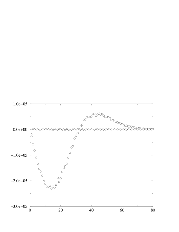
Figure 1: Branched polymer.

This example illustrates the power of the proposed algorithm. We can see that a strong disconnected signal is reduced almost completely and that we are left with only local correlation at $r=0$.

Similar effect is presented on the figure 2 for pure 2d gravity using the data from the combinatorial spherical surfaces with regular triangulations and with 8000 points. The definition of a distance used in this measurement is different than in the discussion presented in the section 2. Instead of the distance between the $\phi^{3}$ vertices (centers of the triangles of the surface), defined in terms of dual links, we use the distance between the vertices of the surface, defined as a shortest path following the links of a surface. We measure the connected correlator of the orders of two vertices (numbers of triangles containing this vertex). This example shows that also in this case we observe the anomalous long-range behavior if the the connected correlator is defined using (2.3). Using an improved definition (2.3) we observe a nontrivial correlation only for very small $r$.

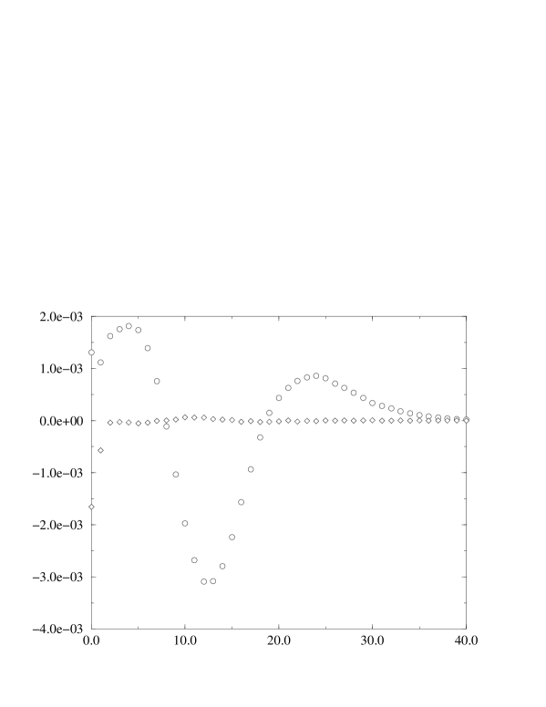
Figure 2: 2d gravity.

We used the same method to study the spin-spin correlations for the ferromagnetic Ising model in a non-zero magnetic field $H$ on a random lattice. This is an example of a theory with a non-trivial matter content. The action for the spin sector of the theory is chosen as

$$S_{I}=-\sum_{\{s_{i}\}}\big{(}\sum_{i,j}\beta\delta_{s_{i},s_{j}}+\sum_{i}H~{}s_{i}\big{)}.$$ (63)

The spins are placed in the centers of triangles and we use degenerate triangulations which allow the two vertices to be connected by more than one link and the links connecting a vertex to itself. This model was solved in [15]. For $H>0$ the model is always in the ordered phase with the geometric properties of pure gravity ($\gamma_{str}=-1/2$ and $d_{h}=4$). For $H=0$ the model has two phases depending on the value of $\beta$. For $\beta=\beta_{c}=-\log((2\sqrt{7}-1)/27)$ it undergoes a third order phase transition between an ordered and a disordered phase. At the transition the geometric properties change ($\gamma_{str}=-1/3$). In our experiment we measure the correlation between $\phi_{i}=(1+s_{i})/2$, (which is 1 for up spin and zero for the down spin). This choice avoids problems close to $H=0$, where $\left\langle s_{i}\right\rangle\to 0$ for every $\beta$ on a finite lattice. In our case $\left\langle\phi_{i}\right\rangle\to 1/2$. The connected correlator is independent on the additive constant and is (up to a trivial factor 1/4) simply the spin-spin correlation function. The distance used is the triangle distance, i.e. the shortest path on a dual lattice. We can predict that if the algorithm works, the observed shift $\delta(H)$ should vanish both for large $H$ and for $H\to 0$. For large $H$ the system becomes completely ordered and the correlation function $G_{N}^{\phi\phi}(r)$ becomes equal to $G_{N}^{11}(r)$. For $H\to 0$ average spin approaches zero and $G_{N}^{1\phi}(r)\approx{1\over 2}G_{N}^{11}(r)$. Below we show results from numerical experiments for system sizes 2k, 4k, 8k and 16k triangles performed at $\beta=\beta_{c}$ for various values of the magnetic field $H$. Similar extensive experiments at $H=0$ were performed by [18], although the definition of distance was different.

On figure 3 we present the connected correlation functions $G_{N}^{\phi\phi}(r)$ versus $r$ for a “large” magnetic field $H=0.0125$ defined in the standard way (2.3). On this and consecutive plots we use colors to distinguish the system size: black for 2k, red for 4k, green for 8k and blue for 16k. We see a large disconnected contribution, which in fact becomes stronger with increasing the system size.

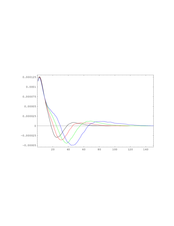
Figure 3: Spin-spin correlation functions at $H=0.0125$ defined by (2.3).

On the next plot we show the same functions scaled by a factor $N^{3/d_{h}-1}$ with $d_{h}=4$ plotted versus the scaling variable $x=(r+\delta_{0})/N^{1/d_{h}}$.

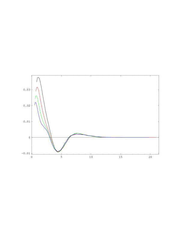
Figure 4: Scaled spin-spin correlation functions at $H=0.0125$

For the sake of presentation we decided to use the theoretical value $d_{h}=4$ rather than to fit this value. The shift $\delta_{0}$ was obtained by matching the scaling of the $G_{N}^{11}(r)$ correlators, again assuming $d_{h}=4$. As we can see the long-range part of the correlator scales exactly as predicted by (2.3). After reduction by (2.3) the correlators contain only the non-scaling part. We show it in figure  5. The shift $\delta(H)=.35\pm.02$ is for this value of $H$ practically independent of the system size.

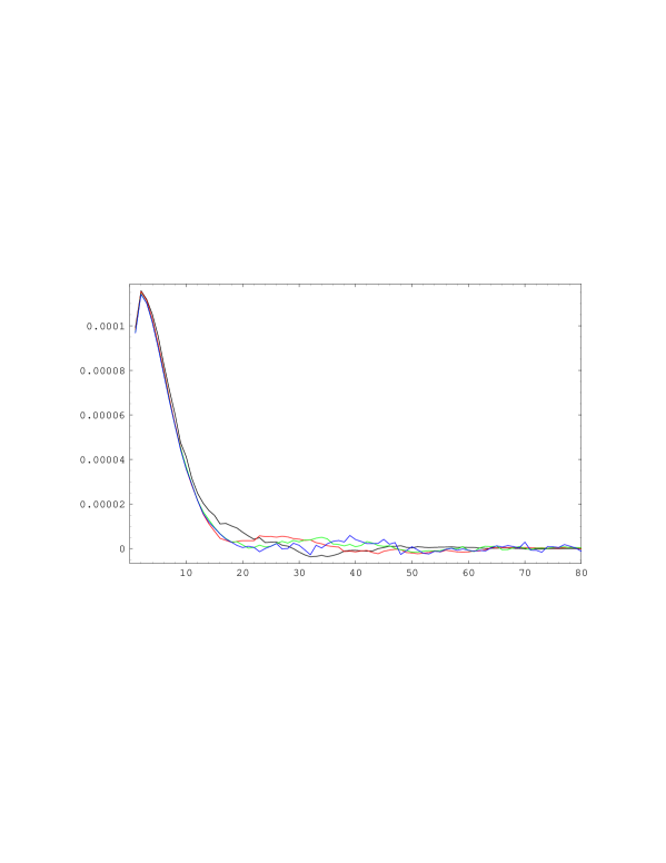
Figure 5: Spin-spin correlation functions at $H=0.0125$ defined using (2.3)

Decreasing the magnetic field $H$ brings us closer to the phase transition. When we apply the algorithm presented above we discover that for each volume the shifts first grow, and then decrease back to zero. The value of the shift as well as the position of the turn over point start to depend on a system volume. From the scaling arguments we expect that near the critical point we should observe a universal behavior of spin-spin correlations, provided the magnetic field is taken as volume dependent in the following way

$$H=\frac{h}{N^{5/6}}.$$

On figure 6 we plot shifts $\delta_{N}(h)$ for the four system sizes. We see that the position of the turn-over point corresponds roughly to $h=1$. Dashed lines join points with the same value of $H$.

Figure 6: Shift $\delta(h)$ vs. $h$.

Below $h=1$ we observe also a change of $\gamma_{str}$ from the pure 2d gravity value $-1/2$ to the $c=1/2$ value $\gamma_{str}=-1/3$. We measured this parameter using the standard method of measuring the minbu distribution [19, 20].

Figure 7: Parameter $\gamma_{str}$ vs. $h$.

Finally figure 8 represents the correlation functions $G_{N}^{\phi\phi,conn}$ obtained using the improved formula (2.3), scaled by a factor $N^{1/d_{h}+1/3-1}$ and plotted versus the scaling variable $x=(r+\delta_{0})/N^{1/d_{h}}$. Values of $d_{h}=4$ and $\delta_{0}=4.5$ are the same as for other plots. Plots correspond from top to bottom to different values of the scaled magnetic field $h=0.2,0.4,\dots 2.0$. The distributions were obtained in practice by interpolating the measured correlation functions at weak fields $H$ to match the scaled values $h$.

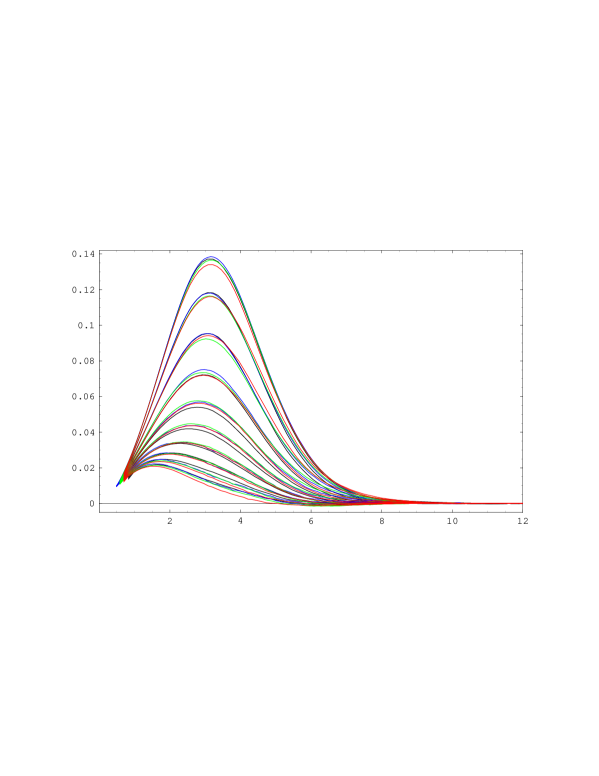
Figure 8: Extrapolated spin-spin correlation functions for (from top to bottom) $h=0.2,~{}0.4,~{}\dots,~{}2.0$

Indeed we observe scaling as predicted.

4 Discussion

A reasonable definition of a connected correlator is given by eq. (1) for a fixed cosmological constant, and by eq. (1) for a fixed space-time volume. However, even when no correlations exist for fixed cosmological constant, the naive discretized analogue of (1), as defined by eq. (2.3), has a non-trivial scaling. This is made explicit in eq. (2.3). Basically a dominant disconnected part is still present in the definition (2.3). As we showed, the refined definition (2.3) manages to cancel this dominant disconnected part and leaves the genuine connected part of the correlator as the dominant part of the two-point correlation.

References

- [1] J. Ambjørn and Y. Watabiki: Nucl. Phys. B 445 (1995) 129-144, hep-th/9501049.
- [2] H. Aoki, H. Kawai, J. Nishimura, A. Tsuchiya, Nucl.Phys.B474 (1996) 512. hep-th/9511117.
-
[3]
B. De Bakker and J. Smit, Nucl.Phys. B454 (1995) 343.
hep-lat/9503004.
B. De Bakker and J. Smit, Nucl.Phys.Proc.Suppl.47 (1996) 613. hep-lat/9510041.
B. De Bakker and J. Smit, Nucl.Phys. B484 (1997) 476. hep-lat/9604023. - [4] P. Bialas, Z. Burda, A. Krzywicki and B. Petersson, Nucl.Phys. B472 (1996) 293.
-
[5]
P. Bialas, Phys. Lett. B373 (1996) 289.
P. Bialas, Nucl. Phys. Proc. Suppl. 53 (1997) 739. hep-lat/9608029. -
[6]
J. Ambjorn, B. Durhuus, J. Frohlich, P. Orland
Nucl. Phys. B270 (1986) 457.
J. Ambjorn, B. Durhuus, T. Jonsson, Phys. Lett. B244 (1990) 403. - [7] P. Bialas, Z. Burda and J. Jurkiewicz: Phys. Lett. B421 (1998) 86, hep-lat/9710070.
- [8] J. Ambjørn, J. Jurkiewicz and Y. Watabiki: Nucl. Phys. B 454 (1995) 313-342, hep-lat/9507014; J. Math. Phys. 36 (1995) 6299-6339, hep-th/9503108.
- [9] J. Jurkiewicz, Acta Phys. Polon. 27 (1996) 1827; hep-lat/9602023
- [10] H. Kawai, N. Kawamoto, T. Mogami and Y. Watabiki, Phys.Lett. B306 (1993) 19. hep-th/9302133
- [11] Y. Watabiki, Nucl.Phys. B441 (1995) 119. hep-th/9401096.
- [12] J. Ambjørn, K. Anagnostopoulos, T. Ichihara, L. Jensen, N. Kawamoto, Y. Watabiki, K. Yotsuji, Nucl.Phys. B511 (1998) 673; hep-lat/9706009
- [13] J. Ambjørn and J. Jurkiewicz, Nucl.Phys. B451 (1995) 643; hep-th/9503006
-
[14]
J. Ambjørn, K.N. Anagnostopoulos, U. Magnea and G. Thorleifsson,
Phys.Lett. B388 (1996) 713.
J. Ambjørn, K.N. Anagnostopoulos, T. Ichihara, L. Jensen, N. Kawamoto, Y. Watabiki and K. Yotsuji, Phys.Lett. B397 (1997) 177; hep-lat/9611032
J. Ambjørn, K.N. Anagnostopoulos, Nucl.Phys. B497 (1997) 445;
hep-lat/9701006. - [15] D.V. Boulatov and V.A. Kazakov, Phys. Lett. B186 (1987) 379.
- [16] E.Brézin, C.Itzykson, G.Parisi and J.B.Zuber, Comm. Math.Phys. 59 (1978) 35.
- [17] J. Ambjørn, K. Anagnostopoulos and J. Jurkiewicz, in preparation.
- [18] J. Ambjørn, K. Anagnostopoulos and U. Magnea, Phys.Lett. B388 (1996) 713.
- [19] J. Ambjorn, S. Jain and G. Thorleifsson, Phys.Lett.B307 (1993) 34. hep-th/9303149.
- [20] J. Ambjorn, S. Jain, J. Jurkiewicz, C.F. Kristjansen, Phys.Lett. B305 (1993) 208. hep-th/9303041.