On the Universality Class of Monopole Percolation
in Scalar QED

Abstract

We study the critical properties of the monopole-percolation transition in U(1) lattice gauge theory coupled to scalars at infinite ($\beta=0$) gauge coupling. We find strong scaling corrections in the critical exponents that must be considered by means of an infinite-volume extrapolation. After the extrapolation, our results are as precise as the obtained for the four dimensional site-percolation and, contrary to previously stated, fully compatible with them.

Keywords: Lattice. Monte Carlo. Percolation. Critical exponents. Phase transitions. Finite-size scaling. QED.

PACS: 11.15.Ha 12.20.-m 14.80.Hv

1 Introduction

The richness of the phase diagram of models containing charged scalars and/or fermions and abelian gauge fields has produced the hope of finding a non-trivial critical point in four dimensions. For the compact formulation of lattice QED, the different phases of these models (Confining, Higgs, Coulomb), can be characterized in terms of their topological content [1], and this relation can be numerically explored [2] (see Ref. [3] for a detailed exposition). The link between topology and phase-diagram is strong to the point that a monopole-percolation second-order phase transition can be found beyond the end-point of the Higgs-Coulomb phase transition line (see Ref. [4] for a study of the phase-diagram). In Ref. [5], it has been conjectured that the monopole-percolation phase transition can produce a chiral phase transition that, being driven by the monopole percolation, would present the same critical exponents.

This conjecture has been put to test in Ref. [3], where the position of both the monopole-percolation and chiral critical lines have been located, by means of a Monte Carlo simulation in the quenched approximation. The chiral critical line is very close to the monopole-percolation one, but they can be clearly resolved in the limit of infinite ($\beta=0$) gauge coupling. A clear-cut test of the scenario proposed in Ref. [5] would be an accurate measure of both the chiral and monopole-percolation critical exponents. The critical exponents for monopole-percolation have been measured in Refs. [3, 6]. The critical exponents displayed a very mild variation along the critical line, consistent with a single Universality Class, although significantly different from the site-percolation [7]. However, in Refs. [3, 6] the scaling corrections are not considered in the analysis.

In this letter, we report the results of a Monte Carlo calculation of compact scalar QED in the strong coupling limit for the gauge field ($\beta=0$), where the model is integrable. In this way, we are able to directly generate independent configurations obtaining accurate measures in large lattices.

In our study, we shall use a Finite-size Scaling (FSS) method based on the comparison of measures taken in two lattices, at the coupling value for which a renormalization group invariant (namely the correlation length in units of the lattice size) takes the same value in both lattices [7, 8, 9]. In this way, by considering the scaling of other dimensionless quantities, we obtain direct information on corrections to scaling. In the present case the scaling corrections are notoriously difficult to deal with. The usual strategy of just considering the leading scaling corrections would only work in extremely large lattices, and we are compelled to use sub-leading corrections in the infinite volume extrapolation. After this extrapolation, we conclude that monopole-percolation belongs to the same Universality Class that site-percolation.

2 The model

The action for the (compact) U(1)-gauge model on the lattice, coupled to unit modulus scalars can be written as

$$S=-\beta\sum_{\mathitbf{r},\mu<\nu}\mathrm{Re}\,U_{\mu\nu}(\mathitbf{r})-\kappa\sum_{\mathitbf{r},\mu}\mathrm{Re}\,\Phi^{\dagger}(\mathitbf{r})U_{\mu}(\mathitbf{r})\Phi(\mathitbf{r}+{\mbox{\boldmath$\mu$}})\ ,$$ (1)

where $\mathitbf r$ is the four-dimensional lattice site, $\mu$ and $\nu$ run over the four spatial directions, $\mu$ is the vector joining neighbours along the $\mu$ direction, $U_{\mu\nu}(\mathitbf{r})$ is the elementary plaquette, $U_{\mu}(\mathitbf{r})$ the gauge variable, and $\Phi(\mathitbf{r})$ the scalar field. The lattice volume is $V=L^{4}$ and periodic boundary conditions are imposed. Notice that we use the normalization of the parameter $\kappa$ as in Ref. [4] which is twice that used in Ref. [3].

For $\beta=0$ and after a gauge transformation to eliminate the $\Phi$ fields, the action simplifies to

$$S=-\kappa\sum_{\mathitbf{r},\mu}\mathrm{Re}\,U_{\mu}(\mathitbf{r})\ .$$ (2)

The generation of independent Monte Carlo configurations for this action is straightforward, as the link variables are dynamically independent.

To study the monopoles in the lattice, let us write $U_{\mu}(\mathitbf{r})=\mathrm{e}^{\mathrm{i}\theta_{\mu}(\mathitbf{r})}$ and define

$$\theta_{\mu\nu}(\mathitbf r)=\theta_{\mu}(\mathitbf r)+\theta_{\nu}(\mathitbf r+{\mbox{\boldmath$\mu$}})-\theta_{\mu}(\mathitbf r+{\mbox{\boldmath$\nu$}})-\theta_{\nu}(\mathitbf r)=\overline{\theta}_{\mu\nu}(\mathitbf r)+2\pi N_{\mu\nu}(\mathitbf r)\ ,$$ (3)

where $\overline{\theta}_{\mu\nu}$ is taken in the interval $(-\pi,\pi]$ and $N_{\mu\nu}$ is an integer.

We obtain the monopole current in the dual lattice as [2]

$$m_{\mu}(\tilde{\mathitbf}r)=\frac{1}{2}\epsilon_{\mu\nu\rho\sigma}\Delta^{+}_{\nu}N_{\rho\sigma}(\mathitbf r+{\mbox{\boldmath$\mu$}})\ ,$$ (4)

where $\Delta^{+}$ is the forward difference operator in the lattice. Each component of the current $m_{\mu}$ is an integer which lives in the link of the dual lattice leaving $\tilde{\mathitbf}r$ in the $\mu$ direction. Clusters are defined as sets of sites of the dual lattice connected through links with nonzero monopole current (occupied links).

The observables that we measure for every gauge configuration are the link energy and magnetization-like quantities that can be expressed in terms of the cluster-size distribution:

$$\begin{array}[]{lcl}E&=&\displaystyle\sum_{\mathitbf{r},\mu}\mathrm{Re}\,U_{\mu}(\mathitbf{r})\ ,\\ M_{1}&=&\displaystyle\sum_{c}n_{c}\ ,\\ M_{2}&=&\displaystyle\sum_{c}n_{c}^{2}\ ,\\ M_{4}&=&\displaystyle 3M_{2}^{2}-2\sum_{c}n_{c}^{4}\ ,\\ \displaystyle M_{\mathrm{max}}&=&\displaystyle\max_{c}n_{c}\ ,\end{array}$$ (5)

where $n_{c}$ is the number of sites of the $c-$nth cluster. $E$ is used to compute $\kappa$ derivatives and to extrapolate the measures taken at $\kappa$ to neighbouring coupling values [10]. The definition of $M_{2}$ ($M_{4}$) can be understood by putting in the occupied sites Ising spins at zero temperature (spins on the same cluster have the same sign), taking the second (fourth) power of the magnetization, and averaging over the signs of the clusters [7].

The same construction allows for a sensible measure of the correlation length in a finite lattice. We first measure the Fourier transform of the clusters

$$\widehat{n}_{c}(\mathitbf{k})=\sum_{\mathitbf{r}\in c}e^{\mathrm{i}\mathitbf{k}\cdot\mathitbf{r}}\,$$ (6)

at minimal momentum, from which we obtain

$$F=\frac{1}{4}\left\langle\sum_{\|\mathitbf{k}\|=2\pi/L}\sum_{c}|n_{c}(\mathitbf{k})|^{2}\right\rangle\ ,$$ (7)

and then use the following definition [11]

$$\xi=\left(\frac{\langle M_{2}\rangle/F-1}{4\sin^{2}(\pi/L)}\right)^{1/2}\ .$$ (8)

We have used two definitions of the unconnected susceptibility

$$\begin{array}[]{lcl}\chi_{1}&=&\langle M_{2}\rangle/V\ ,\\ \chi_{2}&=&\langle M_{\mathrm{max}}^{2}\rangle/V\ .\end{array}$$ (9)

Notice that the monopole density $M_{1}/V$ is not critical at the transition. So, we can define also the susceptibilities dividing $M_{2}$ or $M_{\mathrm{max}}$ by $M_{1}$, as done in Refs. [3, 6]. This should only modify the corrections to scaling (in general, we find that they increase slightly).

The previous numerical studies have been mainly based on measures of connected susceptibilities, specifically

$$\begin{array}[]{lcl}\overline{\chi}_{1}^{\mathrm{c}}&=&\langle(M_{2}-M_{\mathrm{max}}^{2})/M_{1}\rangle\\ \overline{\chi}_{2}^{\mathrm{c}}&=&(\langle(M_{\mathrm{max}}/M_{1})^{2}\rangle-\langle M_{\mathrm{max}}/M_{1}\rangle^{2})V\ .\end{array}$$ (10)

These definitions make sense at both sides of the transition and present a peak near it. However we shall see that they present strong corrections to the scaling, becoming less appropriate than the unconnected ones for a FSS study.

It is also very useful to measure quantities that keep bounded at the critical point, but whose $\kappa$ derivatives diverge. Some examples are the correlation length in units of the lattice size and the Binder parameters:

$$\begin{array}[]{rcl}B_{1}&=&\displaystyle\frac{1}{2}\left(3-\frac{\langle M_{4}\rangle}{\langle M_{2}\rangle^{2}}\right)\ ,\vskip 3.0pt plus 1.0pt minus 1.0pt\\ B_{2}&=&\displaystyle\frac{\langle M_{2}\rangle}{\langle M_{\mathrm{max}}\rangle^{2}}\ ,\vskip 3.0pt plus 1.0pt minus 1.0pt\\ B_{3}&=&\displaystyle\frac{\langle M^{2}_{\mathrm{max}}\rangle}{\langle M_{\mathrm{max}}\rangle^{2}}\ .\end{array}$$ (11)

3 The numerical method

We have simulated in symmetric lattices of linear sizes $L=6,8,12,16,24,32$, and $48$. We have generated $10^{6}$ independent configurations for each lattice. The statistical analysis have been done with 1000 bins of data, for an accurate error determination. To speed up the computations, we have used the U(1) subgroup $Z_{65535}$. We have checked that the U(1)-discretization effects are negligible comparing the results with those using $Z_{255}$.

In order to measure critical exponents, we use a FSS method. Specifically, we use the quotients method used in Refs. [7, 8, 9]. Given an observable $O$ that diverges as $t^{-x_{O}}$, $t$ being the reduced temperature $(\kappa-\kappa_{\mathrm{c}})/\kappa_{\mathrm{c}}$, the FSS ansatz predicts that for a finite lattice of size $L$, in the critical region

$$\langle O(L,t)\rangle=L^{x_{O}/\nu}[F_{O}(\xi(L,t)/L)+O(L^{-\omega})]\ ,$$ (12)

where $F_{O}$ is a smooth scaling function and $\omega$ is the universal exponent associated to the leading corrections to scaling.

To eliminate the unknown function $F_{O}$, one can compute the quotient $Q_{O}$ of the mean value of the observable in two different lattices, at the coupling value where the correlation lengths in units of the lattice size is the same (there is a crossing):

$$\left.Q_{O}\right|_{Q_{\xi}=s}=\frac{\langle O(sL,t_{\mathrm{cross}})\rangle}{\langle O(L,t_{\mathrm{cross}})\rangle}=s^{x_{O}/\nu}+O(L^{-\omega})\ ,$$ (13)

lattice sizes being $sL$ and $L$ respectively. The $O(L^{-\omega})$ terms include all powers of $L^{-\omega}$ as well as the corresponding series produced by sub-leading irrelevant operators [9, 12, 13]. Other corrections are generated by the non singular part of the free energy (analytical corrections). For most observables the analytical corrections are $O(L^{-\gamma/\nu})$. Let us remark that $Q_{O}$ and $Q_{\xi}$ are statistically correlated, which allows for an important (statistical) error reduction in Eq. (13). In fact, a modification of Eq. (13) can be used to study logarithmic corrections to mean-field behaviour with rather high accuracy [14]. Let us finally remark that a similar two-lattices matching method has also being extremely successful in lattice QCD studies [15].

It will be also useful to recall the shift of the finite-lattice critical point from the true critical point [16]:

$$t^{\mathrm{cross}}(L,s)\propto\frac{1-s^{-\omega}}{s^{1/\nu}-1}L^{-\omega-1/\nu}\ ,$$ (14)

where only the leading scaling corrections have been kept. With a fixed value of $s$, $t^{\mathrm{cross}}(L,s)\propto L^{-\omega-1/\nu}$, to be compared with the shift of the peaks of the connected susceptibility, that goes as $t^{\mathrm{peak}}\propto L^{-1/\nu}$. These peaks can be measured in a single lattice, but we loose a factor of $L^{-\omega}$. That is why the quotient method suffers from smaller scaling corrections. Eq. (14) also applies to the crossing of the Binder cumulants $B_{i}$.

4 Results

$L$	$\nu$	$\eta$	$\nu_{\mathrm{s-p}}$	$\eta_{\mathrm{s-p}}$
6	0.6801(34)	$-0.2336(7)$	—	—
8	0.6829(36)	$-0.1713(6)$	0.689(3)	$-0.0687(7)$
12	0.680(5)	$-0.1256(6)$	0.687(3)	$-0.0775(7)$
16	0.681(6)	$-0.1095(7)$	0.688(4)	$-0.0825(6)$
24	0.689(6)	$-0.0986(6)$	0.691(5)	$-0.0868(8)$

Table 1: Critical exponents obtained from Eq.(13) with lattice pairs ($L$,$2L$). We have used as operators $\partial\xi/\partial\kappa$ ($x_{\partial_{\kappa}\xi}=1+1/\nu$), and $\chi_{1}$ ($x_{\chi_{1}}=\gamma/\nu=2-\eta$). The last two rows display the corresponding results for site-percolation (obtained with exactly the same operators) reported in [7].

In table 1 we show our results for the critical exponents $\eta$ and $\nu$ as obtained from Eq. (13). The used operators have been $\chi_{1}$ ($x_{\chi_{1}}=\gamma/\nu=2-\eta$) and $\partial\xi/\partial\kappa$ ($x_{\partial_{\kappa}\xi}=1+1/\nu$). In all cases, we consider only the ratio $s=2$. These exponents can be directly compared with the results for the four dimensional site-percolation [7]. The trend for exponent $\nu$ in both cases is rather similar: the scaling corrections are significantly smaller than the statistical errors, so that the results seems stable with growing $L$. To this accuracy, both measures are compatible. On the other hand, for the anomalous dimension, $\eta$, both systems present significant scaling corrections, although stronger in the monopole-percolation case. Therefore, the scaling corrections must be dealt with before comparison for $\eta$ can be attempted.

In previous studies [7, 8, 9], we have used Eq. (14) to obtain an estimate of $\omega$ that allows to perform an infinite-volume extrapolation. However, in this case the higher-order scaling corrections are so large that they need to be considered. This can be seen in figure 2, where we show the finite-lattice critical point as obtained by the crossing of $\xi/L$, and of $B_{i}$. In the $\xi/L$ case, the behaviour is not even monotonous with increasing lattice size. Therefore, in this problem we need to go beyond Eq. (14).

Thus, we have considered the three Binder cumulants $B_{i}$ whose quotients should behave as

$$\left.Q_{B_{i}}\right|_{Q_{\xi}=s}=1+A_{i}L^{-\omega}+B_{i}L^{-2\omega}+C_{i}L^{-\omega^{\prime}}+D_{i}L^{-\gamma/\nu}+\ldots\ ,$$ (15)

where $\omega^{\prime}$ stands for a sub-leading irrelevant exponent.

Our numerical results for these quotients are plotted in figure 1. Although the behaviour with growing $L$ is not monotonous, we have first considered the parametrization $1+A_{i}L^{-\omega}$, which should be adequate for large $L$. The quality of the fit is rather poor unless discarding all but the two largest pairs: $\omega=0.81(2)\ (\chi^{2}/\mathrm{dof}=159/8)$; $\omega=0.99(5)\ (\chi^{2}/\mathrm{dof}=19.9/5)$; $\omega=1.03(8)\ (\chi^{2}/\mathrm{dof}=5.2/2)$, for $L\geq 8$, $L\geq 12$ and $L\geq 16$ respectively (“dof” is the number of degrees of freedom in the fit). We see that higher-order corrections need to be included. As $\omega$ seems slightly larger than one and, from table 1 it is clear that $\gamma/\nu$ will be close to two, $L^{-2\omega}$ and $L^{-\gamma/\nu}$ will be of the same order. Therefore, a quadratic fit in $L^{-\omega}$ should be a good parametrization provided that there are not sub-leading irrelevant operators in the intermediate range. In fact, the quadratic fit shown in figure  1 (discarding the smaller lattice, $L=6$) is quite reasonable:

$$\omega=1.23(8),\quad\chi^{2}/\mathrm{dof}=5.4/5\ .$$ (16)

Notice that the data used in the fits are strongly correlated and the consideration of the full covariance matrix is mandatory.

A cross-check of the determination Eq. (16) can be done fitting to the functional form $1+A_{i}L^{-\omega}+C_{i}L^{-\gamma/\nu}$, fixing $\gamma/\nu=2.09$ (this is the value found in Ref. [7], for site-percolation and it is also quite close to the values encountered in table 1). This fit yields a compatible value with a rather increased error: $\omega=1.36(14)$.

Therefore, our estimate seems consistent although one may prefer to double the error in Eq. (16), as an estimation of systematic errors, to be in the safe side.

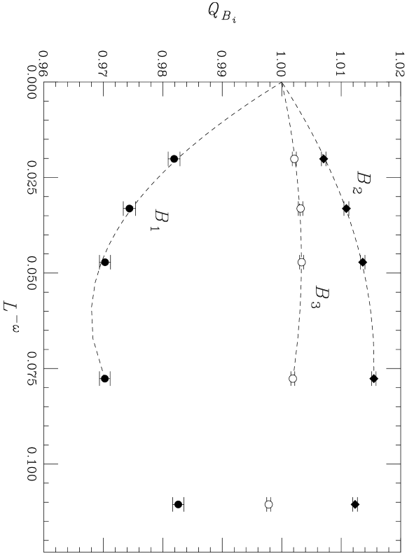
Figure 1: Quotients of cumulants $B_{1}$, $B_{2}$ and $B_{3}$ as a function of $L^{-\omega}$. We use for $\omega$ the value obtained in the fit, thus the curvature is related with higher-order corrections to scaling.

A different cross-check is the infinite-volume extrapolation for $\kappa_{\mathrm{c}}$, using Eq. (14) and the crossing points for $\xi/L,B_{1},B_{2}$ and $B_{3}$. In figure 2 we plot the cumulant crossing points as a function of $L^{-\omega-1/\nu}$. As the behaviour is not monotonous we have tried a fit to $\kappa_{\mathrm{c}}+A_{i}L^{-\omega-1/\nu}+B_{i}L^{-2\omega-1/\nu}$. From table 1 and Eq. (16) we find that $\nu$ can be determined much more accurately than $\omega$, so its value can be safely fixed to $\nu=0.69$ in the fit. Fixing also $\omega$ to (16) we obtain an acceptable fit only if $L\geq 12$ ($\chi^{2}/\mathrm{dof}=1.1/3$). We obtain

$$\kappa_{\mathrm{c}}=2.698736(34)(11)\ .$$ (17)

Through out the paper the second error will denote the error induced by the uncertainty in $\omega$. Therefore, if one chooses to double the error in $\omega$, this second error needs to be doubled too. As the value of $\kappa_{\mathrm{c}}$ will be by far our most precise result, it is important to check that the discretization effect of using $Z_{65535}$ instead of U(1) is negligible. In order to do so, we have repeated the measure of the crossing point for the pair $(12,24)$ using $Z_{255}$ with the same statistics, obtaining a compatible value within errors (one per million).

Figure 2: Crossing points of the cumulants, as functions of $L^{-\omega-1/\nu}$ (here we have set $\omega=1.23$, $\nu=0.69$).

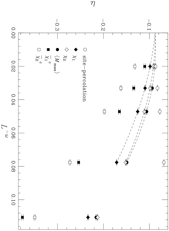
Figure 3: The exponent $\eta$ as a function of $L^{-\omega}$ for several magnetization or susceptibility operators. The dashed lines are quadratic fits in the variable $L^{-\omega}$ ($\omega=1.23$). Notice that the connected susceptibilities present stronger scaling corrections. We also plot the results of the site-percolation taken from Ref. [7].

The exponent $\eta$ can be obtained from the susceptibilities $\chi_{1}$ and $\chi_{2}$ (which scale as $L^{\gamma/\nu}=L^{2-\eta}$) and the magnetization $\langle M_{\mathrm{max}}\rangle$ (which scales as $L^{-\beta/\nu+4}=L^{3-\eta/2}$). In figure 3, we show the three $\eta$ determinations. It is clear from the plot that we cannot keep just the leading scaling corrections. In this figure we show a joint fit of the three quantities, quadratic in $L^{-\omega}$, with $L\geq 8$. The extrapolated value is

$$\eta=-0.0876(22)(6),\quad\chi^{2}/\mathrm{dof}=1.2/5\ .$$ (18)

This might be compared with the result obtained by assuming that the scaling corrections are $A_{i}L^{-\omega}+C_{i}L^{-\gamma/\nu}$ (fixing again $\gamma/\nu=2.09$):

$$\eta=-0.0902(25)(1),\quad\chi^{2}/\mathrm{dof}=2.4/5\ .$$ (19)

We see that by following our recipe of doubling the $\omega$ induced error, both extrapolations are not covered by the second error bar. We thus take the difference to estimate the systematic error involved in the infinite-volume extrapolation generated by higher-order terms. The final value that includes both kind of errors is

$$\eta=-0.089(4)\ .$$ (20)

For computing the $\nu$ exponent we measure the quotient corresponding to the operator $\partial\xi/\partial\kappa$, which scales as $L^{1+1/\nu}$. From table 1 we see that the infinite-volume extrapolation is not so crucial in this case. However, we cannot just average the different determinations (which is basically what a log-log fit does), as the statistical error in the mean can decrease enough to uncover the scaling corrections. In order to obtain a safe error estimate, we perform a fit linear in $L^{-\omega}$. The difference between the extrapolation with $L\geq 6$ and with $L\geq 8$ is ten times smaller than the error. Taking the error from the latter we obtain:

$$\nu=0.685(6),\quad\chi^{2}/\mathrm{dof}=1.0/3\ .$$ (21)

In this case, the $\omega$-induced error is twenty times smaller than the statistical error.

We summarize the infinite-volume extrapolation of critical exponents and of the critical coupling in table 2.

Source	$\kappa_{\mathrm{c}}$	$\nu$	$\eta$	$\omega$
This work	2.69874(6)	0.685(6)	$-0.089(4)$	1.23(16)
Franzki, Kogut, Lombardo [3]	2.6938(8)	0.61(4)	$-0.28(2)$	—
Site-percolation [7]	—	0.689(10)	$-0.094(3)$	1.13(10)

Table 2: Summary of the values obtained for the critical coupling including statistical and our estimation of systematic errors. In the second row we show the results of Ref. [3] for the same system. Finally (third row) we recall the results of Ref. [7] for the site-percolation.

5 Conclusions

We have studied with Finite-size Scaling techniques the monopole percolation transition of compact QED coupled to scalars in the strong-coupling limit ($\beta=0$). We have shown that state of the art techniques for measuring critical exponents in spin models can be successfully applied to this problem. The approach relies in comparison of measures taken in two different lattices when a matching condition is fulfilled (see Eq. (13)). The efficiency of the method is greatly enhanced by the availability of a re-weighting method [10], and of an easily measurable Renormalization Group invariant (the correlation length in units of the lattice size [11]).

With the achieved accuracy in individual measures, the scaling corrections for the reachable lattice sizes are big enough to require the consideration of sub-leading scaling-corrections in the infinite-volume extrapolation. After this extrapolation, it is found (within errors) that at $\beta=0$ monopole-percolation and site-percolation belong to the same Universality Class. The discrepancy with previous calculations is explained by the presence of strong corrections to scaling.

The present study can be extended to the monopole-percolation critical line at non-zero $\beta$ coupling [3, 6], although the number of independent configurations that could be generated would be quite smaller. Another interesting matter is the comparison with the chiral critical behaviour. Our method would be useful in this respect only if it is found an analogous of the correlation length in a finite lattice, that made sense at (chiral) criticality.

References

- [1] M. B. Einhorn and R. Savit, Phys. Rev. D 17 (1978) 2583; Phys. Rev. D 19 (1979) 1198; T. Banks, R. Myerson and J. Kogut, Nucl. Phys. B 129 (1977) 493;
- [2] T. A. DeGrand and D. Toussaint, Phys. Rev. D 22 (1980) 2478; J. Barber, R. Shrock and R. Schrader, Phys. Lett. B 152 (1984) 221; J. Barber and R. Shrock, Nucl. Phys. B 257 (1985) 515; M. Baig, H. Fort and J.B. Kogut, Phys. Rev. D 50 (1994) 5920.
- [3] W. Franzki, J.B. Kogut and M.P. Lombardo, Phys. Rev. D 57 (1998) 6625.
- [4] J.L. Alonso et al, Nucl. Phys. B 405 (1993) 574.
- [5] J. B. Kogut and K. C. Wang, Phys. Rev. D 53 (1996) 1513.
- [6] M. Baig and J. Clua, Phys. Rev. D 57 (1998) 3902.
- [7] H. G. Ballesteros, L. A. Fernández, V. Martín-Mayor, A. Muñoz Sudupe, G. Parisi and J. J. Ruiz-Lorenzo, Phys. Lett. B 400 (1997) 346.
- [8] H. G. Ballesteros, L.A. Fernández, V. Martín-Mayor, and A. Muñoz Sudupe, Phys. Lett. B 378 (1996) 207; Phys. Lett. B 387 (1996) 125; Nucl. Phys. B 483 (1997) 707.
- [9] H. G. Ballesteros, L. A. Fernandez, V. Martín-Mayor, A. Muñoz Sudupe, G. Parisi and J. J. Ruiz-Lorenzo, cond-mat/9805125, to be published in J. Phys. A.
- [10] M. Falcioni, E. Marinari, M. L. Paciello, G. Parisi and B. Taglienti, Phys. Lett. B 108 (1982) 331; A. M. Ferrenberg and R. H. Swendsen, Phys. Rev. Lett. 61 (1988) 2635.
- [11] F. Cooper, B. Freedman and D. Preston, Nucl. Phys. B 210 (1989) 210.
- [12] M. N. Barber, Finite-size Scaling in Phase Transitions and Critical phenomena, edited by C. Domb and J.L. Lebowitz (Academic Press, New York, 1983) vol 8.
- [13] H.W.J. Blöte, E. Luijten and J. R. Heringa, J. Phys. A28 (1995) 6289.
- [14] H.G. Ballesteros, L.A. Fernández, V. Martín-Mayor, A. Muñoz Sudupe, G. Parisi and J.J. Ruiz-Lorenzo, Nucl. Phys. B 512 (1998) 681;
- [15] M. Lüscher, P. Weisz, R. Sommer, U. Wolff, Nucl. Phys. B 389 (1993) 247; K. Jansen, C. Liu, M. Lüscher, H. Simma, S. Sint, R. Sommer, P. Weisz, U. Wolff, Phys. Lett. B 372 (1996) 275.
- [16] K. Binder, Z. Phys. B 43 (1981) 119.