Dublin Preprint: TCDMATH 98-14

The Phase Structure of the Weakly
Coupled Lattice Schwinger Model
R. Kenna,
School of Mathematics, Trinity College Dublin, Ireland
 
C. Pinto and J.C. Sexton
School of Mathematics, Trinity College Dublin, Ireland
and
Hitachi Dublin Laboratory, Dublin, Ireland

December 1998

The weak coupling expansion is applied to the single flavour Schwinger model with Wilson fermions on a symmetric toroidal lattice of finite extent. We develop a new analytic method which permits the expression of the partition function as a product of pure gauge expectation values whose zeroes are the Lee–Yang zeroes of the model. Application of standard finite–size scaling techniques to these zeroes recovers previous numerical results for the small and moderate lattice sizes to which those studies were restricted. Our techniques, employable for arbitrarily large lattices, reveal the absence of accumulation of these zeroes on the real hopping parameter axis at constant weak gauge coupling. The consequence of this previously unobserved behaviour is the absence of a zero fermion mass phase transition in the Schwinger model with single flavour Wilson fermions at constant weak gauge coupling.

Introduction

In lattice gauge theory, there has been considerable discussion on the phase structure of gauge theories with Wilson fermions. A system of free Wilson fermions exhibits a second order phase transition at $(\beta,\kappa)=(\infty,1/(2d))$, $\beta$ and $\kappa$ being the usual inverse gauge coupling squared and hopping parameters respectively and $d$ being the lattice dimensionality. Recent discussions concern the extent to which this phase transition extends into the $(\beta,\kappa)$ plane, the expectation being that there is a line of phase transitions (the chiral limit) extending to the strong coupling limit $\beta=0$. In the simplest model to which this applies, the lattice Schwinger model [1], there is also a second order phase transition in the strongly coupled limit [2]. This critical line, which is expected to connect these two phase transitions, is also expected to recover massless physics and therein lies the importance in determining its nature and position.

While earlier numerical results casted doubt on the above scenario [3], more recent ones support the hypothesis that the critical line extends over the whole range of couplings [4, 5, 6]. To our knowledge, only two groups have attempted to determine the phase diagram in the lattice Schwinger model. While in rough agreement regarding the location of the critical line, they differ in their conclusions regarding its quantitive critical properties. Using Lee–Yang zeroes [7], finite–size scaling techniques [8] as well as PCAC relations, the results of [4, 5] support the free boson scenario, where the model lies in the same universality class of the Ising model, with correlation length critical exponent $\nu=1$ and the specific heat (chiral susceptibility) exponent $\alpha=0$. This is not in agreement with [6] where finite–size scaling of Lee–Yang zeroes on larger lattices provides evidence for $\nu=2/3$, $\alpha=2/3$.

The precise analytical determination of the phase structure in the weakly coupled regime is the primary motivation for this work. We contend that the Lee–Yang zeroes in the Schwinger model with fixed weak gauge coupling display very unusual size–dependent behaviour, do not accumulate on the real hopping parameter axis and may not, in fact, lead to a phase transition. The behaviour of these zeroes is, however, such as to mimic the appearance of a phase transition when a finite–size analysis is restricted to small or moderate lattice sizes.

Lattice Schwinger Model

We consider a finite $d=2$ dimensional lattice with spacing $a$ and $N$ sites in each direction. For the fermion fields, we impose antiperiodic boundary conditions in the temporal ($1$-) direction and periodic boundary conditions in the spatial ($2$-) direction. Lattice sites are labelled $x_{\mu}=n_{\mu}a$ where $n_{\mu}=-N/2,\dots,N/2-1$. With these mixed boundary conditions the momenta for the Fourier transformed fermion fields are $k_{\mu}=2\pi{\hat{k}}_{\mu}/Na$, where ${\hat{k}}_{1}=-N/2+1/2,\dots,N/2-1/2$ and ${\hat{k}}_{2}=-N/2,\dots,N/2-1$.

The action for gauge invariant lattice QED with Wilson fermions is $S_{\rm{QED}}=S_{G}[\phi]+S_{F}^{(W)}[\phi,\psi,\bar{\psi}]$, where $S_{F}^{(W)}[\phi,\psi,\bar{\psi}]=\sum_{m,n}\bar{\psi}(m)M^{(W)}(m,n)\psi(n)$ and

$$M^{(W)}(m,n)=\frac{1}{2\kappa}\delta_{m,n}-\frac{1}{2}\sum_{\mu}{\left\{(r-\gamma_{\mu})U_{\mu}(m)\delta_{m+\hat{\mu},n}+(r+\gamma_{\mu})U^{\dagger}_{\mu}(n)\delta_{m-\hat{\mu},n}\right\}}\quad.$$ (1)

This Wilson fermion matrix can be written in terms of free and interacting parts as $M^{(W)}=M^{(0)}+M^{({\rm{int}})}$ where $M^{(0)}$ is given by $U_{\mu}=1$ in (1). Here $U_{\mu}(n)=\exp{i\phi_{\mu}(n)}=\exp{(ie_{0}aA_{\mu}(n))}$ is the link variable. The Wilson parameter, $r$, is henceforth set to unity. The partition function is $Z_{\rm{QED}}=\int{{\cal{D}}U{\cal{D}}\bar{\psi}{\cal{D}}\psi\exp{(\{-S_{\rm{G}}-S^{(W)}_{\rm{F}}\})}}\propto\int{{\cal{D}}U\exp{\{-S_{\rm{G}}\}}\det{M^{(W)}}}\propto\langle\det{M^{(W)}}\rangle$, the integration over the Grassmann Fermionic fields having been performed. Here $\langle{\cal{O}}\rangle$ is the pure gauge expectation value of the quantity ${\cal{O}}$ and the pure gauge action is $S_{G}[\phi]=\beta\sum_{P}{\left[1-\frac{1}{2}(U_{P}+U_{P}^{\dagger})\right]}$, where $U_{P}$ is the usual product of link variables around a fundamental plaquette and where $\beta=1/e_{0}^{2}a^{2}$. In the weak coupling expansion we employ the Feynman gauge for the calculation of pure gauge expectation values. (There, for large enough $N$, the gauge propagator in momentum space is given approximately by $\langle\tilde{\phi}_{\mu}(\hat{p})\tilde{\phi}_{\nu}(-\hat{p})\rangle=\delta_{\mu\nu}(N^{d}a^{2d}/2\beta)\sum_{\rho,p\neq 0}{(1-\cos{p_{\rho}a})}$ with the infra–red zero–momentum mode excluded as standard [9].)

For $\beta=\infty$, the only gauge configurations which contribute have $S_{G}=0$. We assume for the following analysis that all gauge configurations satisfying this condition belong to a single equivalence class under the group of gauge transformations. Since the fermion determinant is gauge invariant under the same group of gauge transformations it is sufficient to evaluate the full partition function on this single configuration to determine the behaviour of the system at $\beta=\infty$ [4]. Therefore the partition function is simply proportional to $\det{M^{(0)}}$. Employing lattice Fourier transforms, the free fermion partition function can be written in terms of its $dN^{d}$ eigenvalues by solving the $d\times d$ dimensional eigenvalue problem of the form $M^{(0)}(p)|\lambda^{(0)}_{\alpha}(p)\rangle=\lambda^{(0)}_{\alpha}(p)|\lambda^{(0)}_{\alpha}(p)\rangle$ where $\alpha=1,\dots,d$. In $d=2$ dimensions, the resulting eigenvalues are $\lambda^{(0)}_{\alpha}(p)=1/2\kappa-\sum_{\rho=1}^{2}\cos{p_{\mu}a}+i(-)^{\alpha}\sqrt{\sum_{\rho=1}^{2}{\sin^{2}{p_{\rho}a}}}$.

With mixed boundary conditions, the eigenvalues in the free fermion case are either two–fold ($\hat{p}_{2}=0$ or $-N/2$) or four–fold degenerate. In this case, and with $\eta=1/2\kappa$, the Lee–Yang zeroes are $\eta^{(0)}_{\alpha}(p)=\sum_{\rho=1}^{2}r\cos{p_{\mu}a}-i(-)^{\alpha}\sqrt{\sum_{\rho=1}^{2}{\sin{p_{\rho}a}}}$. The lowest zero with finite real part in $\kappa$ corresponds to $\hat{p}=(\pm 1/2,0)$ and for a symmetric lattice is $\eta^{(0)}_{\alpha}(\pm 1/2,0)=1+\cos(\pi/N)-i(-)^{\alpha}{\sin{(\pi/N)}}$. Pinching of the positive real finite hopping parameter axis occurs at the massless point $\kappa_{c}=1/2d$ and application of finite–size scaling [8] to the imaginary parts of the zero gives the critical exponent $\nu=1$ ($\alpha=0$ then follows from hyperscaling). Therefore the free fermion model is in the same universality class as the Ising model in two dimensions and describes free bosons. In the presence of a gauge field the position and nature of this phase transition will change and a quantitive investigation into the nature of that change is the central aim of this paper.

The Weak Coupling Expansion

The weak coupling expansion is formally obtained by expanding the link variables $U_{\mu}(n)$ as a power series in $e_{0}$. The weak coupling expansion of the matrix $M^{({\rm{int}})}$ in (1) is $M^{({\rm{int}})}=M^{(1)}+M^{(2)}+{\cal{O}}(e_{0}^{3})$ where $M^{(n)}$ is of order $e_{0}^{n}$. The fermion determinant $\det{M^{(W)}}=\det{M^{(0)}}\times\det{{M^{(0)}}^{-1}M^{(W)}}=\det{M^{(0)}}\exp{{\rm{tr}}\ln{(1+{M^{(0)}}^{-1}M^{({\rm{int}})})}}$ can then be expanded giving the following ‘traditional’ additive form for the weak coupling expansion [11]:

$$\frac{\langle\det{M^{(W)}}\rangle}{\det{M^{(0)}}}=1+\sum_{i=1}^{dN^{d}}{\frac{t_{i}}{\eta-\eta_{i}^{(0)}}}-\frac{1}{2}\sum_{i\neq j}^{dN^{d}}{\frac{t_{ij}}{(\eta-\eta_{i}^{(0)})(\eta-\eta_{j}^{(0)})}}+\dots\quad.$$ (2)

in which $t_{i}=\langle M_{ii}^{({\rm{int}})}\rangle$ and $t_{ij}=t_{ji}=\langle M_{ij}^{({\rm{int}})}M_{ji}^{({\rm{int}})}\rangle-\langle M_{ii}^{({\rm{int}})}M_{jj}^{({\rm{int}})}\rangle$. Here the index $i$ generically stands for the combination of Dirac index and momenta $(\alpha,p)$ which label fermionic matrix elements so that $M_{ij}^{({\rm{int}})}$ represents $\langle\lambda_{\alpha}^{(0)}(q)|M^{({\rm{int}})}(q,p)|\lambda_{\beta}^{(0)}(p)\rangle$. We note at this point that the expansion is analytic in $\eta$ with poles at $\eta=\eta_{i}^{(0)}$. We note further that $t_{i}=\langle M_{ii}^{({\rm{int}})}\rangle$ at order $e$ is proportional to the pure gauge expectation value of the gauge field $\phi_{\mu}$ and is zero.

An alternative formulation of the partition function may be obtained by writing the Wilson fermion matrix as $M^{(W)}=\eta+H$ where $H$ is the hopping matrix. The fermion determinant $\det M^{(W)}=\det(\eta+H)$, is a polynomial in $\eta$ since for finite lattice size these matrices are of finite dimension. Therefore the pure gauge expectation value of the fermion determinant is also a polynomial in $\eta$ and as such may be written $\langle\det M^{(W)}\rangle=\prod_{i=1}^{dN^{d}}(\eta-\eta_{i})$. Here $\eta_{i}$ represent $\eta_{\alpha}(p)$ and are the Lee–Yang zeroes in the complex $1/2\kappa$ plane. We may write a ‘multiplicative’ weak coupling expansion as

$$\frac{\langle\det{M^{(W)}}\rangle}{\det{M^{(0)}}}=\prod_{i=1}^{dN^{d}}\frac{(\eta-\eta_{i})}{(\eta-\eta_{i}^{(0)})}=\prod_{i=1}^{dN^{d}}\left(1-\frac{\Delta_{i}}{\eta-\eta_{i}^{(0)}}\right)\quad,$$ (3)

where $\Delta_{i}=\eta_{i}-\eta_{i}^{(0)}$ are the shifts that occur in the zeroes when the gauge field is turned on and are the quantities to be determined. Note again that (3) is analytic in $\eta$ with poles at $\eta_{i}^{(0)}$. Since the two expressions (2) and (3) must be equal, the residues of the poles must be identical.

Let $t_{i}=t_{i}^{(2)}+\dots$, $t_{ij}=t_{ij}^{(2)}+\dots$ and $\Delta_{i}=\eta_{i}^{(1)}+\eta_{i}^{(2)}+\dots$ where $\eta_{i}^{(1)}$ is ${\cal{O}}(e)$ and $t_{i}^{(2)}$, $t_{ij}^{(2)}$ and $\eta_{i}^{(2)}$ are ${\cal{O}}(e^{2})$. Assume the $n_{j}^{\rm{th}}$ free eigenvalues are degenerate for $j=1,\dots,D_{n}$ where $D_{n}$ is $2$ or $4$ and $\lambda^{(0)}_{n_{j}}\equiv\lambda^{(0)}_{n}$. At this stage we make no assumptions regarding the other eigenvalues. The traditional weak coupling expansion (2) and its ‘multiplicative’ counterpart (3) have single poles at $\eta=\eta^{(0)}_{n}$, the residues of which are easily calculated to ${\cal{O}}(e^{2})$. Equating the two residues order by order in $e$ gives

$$\sum_{j=1}^{D_{n}}{\eta_{n_{j}}^{(1)}}=0\quad,\quad\quad\quad\sum_{j=1}^{D_{n}}{\eta_{n_{j}}^{(2)}}=D_{n}\bar{\Delta}_{n}^{(2)}\equiv\sum_{j=1}^{D_{n}}{\left[-t_{n_{j}}^{(2)}+\sum_{i,\lambda_{i}^{(0)}\neq\lambda_{n}^{(0)}}{\frac{t_{in_{j}}^{(2)}}{\eta_{n}^{(0)}-\eta_{i}^{(0)}}}\right]}\quad.$$ (4)

In this latter equation, $\bar{\Delta}_{n}^{(2)}$ is the average of two zeroes which in the free fermion case were two–fold degenerate and is ${\cal{O}}(e^{2})$. Equating the residues of the corresponding double poles gives no extra information at this order.

In the non–degenerate case $D_{n}=1$, (4) is sufficient and necessary to fully determine the shifts in the positions of the zeroes $\eta_{n_{j}}^{(1)}$ and $\eta_{n_{j}}^{(2)}$. This then amounts to a new method to uniquely express the partition function and all derivable thermodynamic functions in multiplicative (as opposed to the traditional ‘additive’) form. Thus, we have expressed the pure gauge expectation value of a product of fermion eigenvalues as a product of pure gauge expectation values.

In the $D_{n}$–fold degenerate case, (4) gives for the expansion of the ‘multiplicative’ weak coupling expression (3) to ${\cal{O}}(e^{2})$,

$$\prod_{i}{\left(1-\frac{\Delta_{i}}{\eta-\eta_{n_{i}}^{(0)}}\right)}=1+\sum_{i}{\frac{t_{i}^{(2)}}{\lambda_{i}^{(0)}}}+\sum_{i,j,\lambda_{i}^{(0)}\neq\lambda_{j}^{(0)}}{\frac{t_{ij}^{(2)}}{\lambda_{i}^{(0)}(\lambda_{i}^{(0)}-\lambda_{j}^{(0)})}+\sum_{i\neq j}{\frac{\Delta_{i}\Delta_{j}}{\lambda_{i}^{(0)}\lambda_{j}^{(0)}}}+\dots}\quad.$$ (5)

This is identical to the traditional weak coupling expansion (2) to ${\cal{O}}(e^{2})$ if

$$\sum_{i}{\left(\frac{\eta_{i}^{(1)}}{\lambda_{i}^{(0)}}\right)^{2}}=\sum_{i\neq j,\lambda_{i}^{(0)}=\lambda_{j}^{(0)}}{\frac{t_{ij}^{(2)}}{\left(\lambda_{i}^{(0)}\right)^{2}}}\quad.$$ (6)

Setting $\eta=\eta_{n}^{(0)}+\epsilon$ where $\epsilon\neq 0$ and separating out the contributions coming from the $D_{n}$–fold degenerate cases $n_{j}$ now gives that

$$\sum_{i=1}^{D_{n}}(\eta_{n_{i}}^{(1)})^{2}=\sum_{i=1}^{D_{n}}\sum_{j=1,j\neq i}^{D_{n}}t^{(2)}_{n_{i}n_{j}}+{\cal{O}}(\epsilon)\quad.$$ (7)

Now the ‘multiplicative’ and ‘additive’ expressions for the partition function coincide up to ${\cal{O}}(e^{2})$ everywhere in the complex $1/2\kappa$ plane arbitrarily close to any pole and have the same poles and the same residues (up to ${\cal{O}}(e^{2})$) at those poles. The partition function zeroes are $\eta_{n_{i}}=\eta_{n}^{(0)}+\eta_{n_{i}}^{(1)}+\bar{\Delta}_{n}^{(2)}$ where in the free field case the ${n_{i}}^{\rm{th}}$ zero is in the $n^{\rm{th}}$ degeneracy class. In terms of the Dirac and momenta labels, we can write the erstwhile 2–fold degenerate lowest zeroes as

$$\eta_{\alpha}(\pm p_{1},0)=\eta_{\alpha}^{(0)}(|p_{1}|,0)\pm\eta_{\alpha}^{(1)}(|p_{1}|,0)+\bar{\Delta}_{\alpha}^{(2)}(|p_{1}|,0)\quad.$$ (8)

In this way, the shifts in the positions of the erstwhile two–fold degenerate zeroes are also determined to ${\cal{O}}(e^{2})$ and the ${\cal{O}}(e^{2})$–shift is the shift in the average position of the two zeroes while their relative separation is ${\cal{O}}(e)$. The calculation of Lee–Yang zeroes is now reduced to the calculation of the pure gauge expectation values $\Delta_{\alpha}(p)$ which we do in Feynman gauge.

Results and Conclusions

The main plot in Figure 1 is a finite–size scaling plot for the lowest zero for $\beta=10$ and $N=8,10,...,62$ coming from our weak coupling analysis (circles). The corresponding data from the numerical analysis of [6] are also included (crosses). The two lines are the linear fit to the lowest zeroes for lattice sizes $16,20,24$ of [6] and a fit to the second zero. These yield slopes $-1.5$ and $-1.4$ respectively, corresponding to $\nu\approx 2/3$. The insert contains a similar plot at $\beta=5$ where the circles are our results for $N=2,4,...,42$ and the squares are the results of [4] for the lowest zero for $N=2,4,8$. The line is the best linear fit to this latter data and yields $\nu$ compatable with $1$. Fitting to our small lattice data also gives $\nu\approx 1$.

Therefore, confining the finite–size scaling analysis to the range $N=2$ – $8$ yields a slope compatable with $\nu=1$ in agreement with [4]. A corresponding analysis with $N=8$–$24$ gives a steeper slope, compatable with $\nu=2/3$ in agreement with [6]. It is clear from the figure, however, that the curve does not in fact settle to a finite–size scaling line. Instead as $N$ increases, the lowest zero crosses the real $1/2\kappa$ axis. The second zero exhibits the same behaviour as demonstrated by the upper curve in Figure 1. The first two zeroes therefore fail to accumulate and do not contribute to critical behaviour [7, 12, 13]. One interprets these zeroes as isolated singularities of thermodynamic functions, having measure zero in the thermodynamic limit.

Figure 1: The finite–size scaling behaviour of the imaginary parts of the first two Lee–Yang zeroes for $\beta=10$. The symbols $\circ$ are our weak coupling expansion results. The numerical results of [6] for $N=8,\dots,24$ are $\times$ and the lines are best fits to these points. The insert is a similar plot for $\beta=5$. There the $\Box$ are the lowest zeroes of [4].

It would be extremely difficult to detect the isolated nature of these Lee–Yang zeroes from numerical data alone. A standard numerical technique for determination of the phase diagram – assuming accumulation of zeroes – is to approximate the infinite volume critical point by the real part of the lowest zero (then a pseudocritical point) for some reasonably large lattice. Plotted against $\beta$ this appproximates the phase diagram. In Figure 2 we present such a plot for $N=24$ (circles) to compare with the results of [6] (crosses) also at $N=24$. The phase diagram of [5] for the Schwinger model with two fermion flavours coming from a separate PCAC based analysis is also included (squares) for comparison.

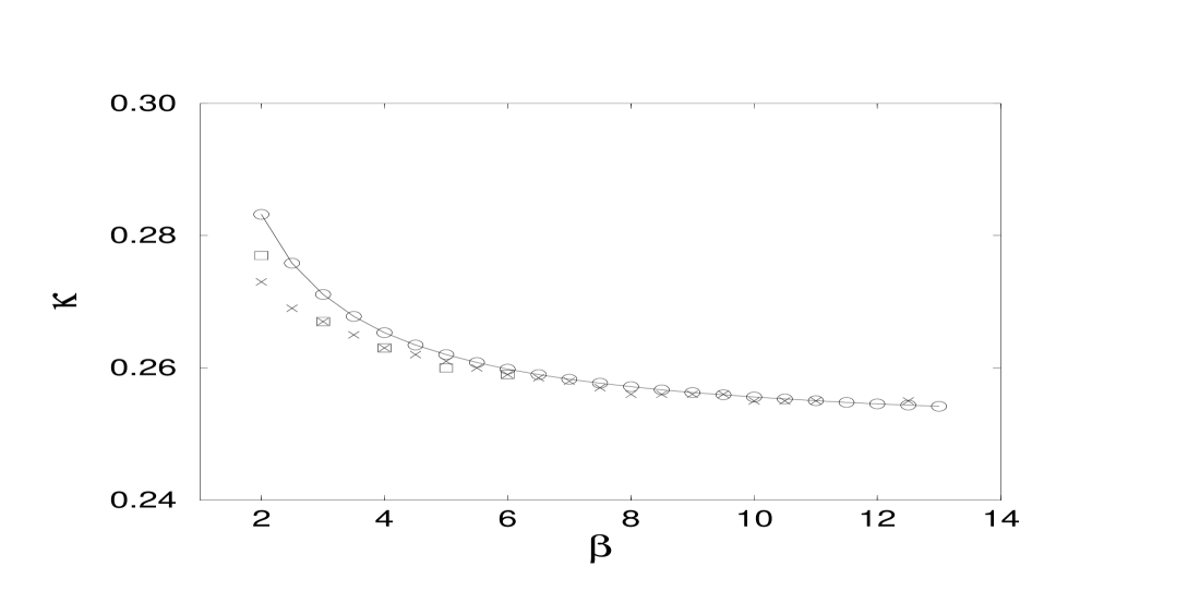
Figure 2: The would–be phase diagram coming from the real parts of the lowest zeroes at various $\beta$ at fixed $N$. The symbols $\circ$ are our weak coupling expansion results for $N=24$ and $\times$ are numerical results of [6] also for $N=24$. The symbols $\Box$  are the numerical results of [5] for $N=16$ and two fermion flavours.

Now, the ${\cal{O}}(e)$ shift in the free field lowest zero is, in fact, $\eta_{\alpha}^{(1)}(\pm 1/2,0)=\pm(i/(Na)^{d})\sqrt{\langle|\phi_{\mu}(1,0)|\rangle}=\pm i/(2\sqrt{\beta}N|\sin{p_{1}a}|)$, the leading finite–size scaling behaviour of which is $N$–independent. The crossing of the real axis by the first two zeroes is therefore due to the $N$ dependency of their ${\cal{O}}(e^{2})$ average. In the four fold degenerate case, the leading $N$ behaviour of the zeroes is again determined by that of their average. The four fold degenerate ${\cal{O}}(e^{2})$ averages of small momentum zeroes also cross the real axis and do not accumulate.

Although we cannot logically exclude the possibility that some zero which was far from the real axis in the free fermion case (or some combination of such zeroes) conspires to accumulate on the real $1/2\kappa$ axis in the usual way, such a situation seems unlikely. Nor can we exclude the possiblilty that just as the subdominant terms in the weak coupling expansion (the ${\cal{O}}(e^{2})$ averages) correspond to the dominant $N$ behaviour, so too could higher order terms in the weak coupling expansion correspond to superdominant $N$ effects. This seems again unlikely as the average zeroes coming from our weak coupling expansion agree very well with those of [6] (see [10] for more details). Moreover, superdominant $N$ effects from subdominant weak coupling terms would spell disaster for lattice (and indeed continuum) perturbation theory and is an unlikely scenario in this – a superrenormalisable – model.

Although the possibility of existence of isolated singularities and non–accumulation of partition function zeroes has been known for a long time [7, 12, 13], this is to our knowledge the first instance where such behaviour has been observed. In conclusion, in the free case, there is a phase transition precipitated by the accumulation of Lee–Yang zeroes on the real hopping parameter axis. In the weakly coupled regime at fixed $\beta$, this accumulation no longer occurs. Instead, the movement of zeroes for small and moderately sized lattices mimics phase transition like behaviour. As the lattice size becomes large, however, these zeroes move across the real axis, and do not give rise to a phase transition.

Acknowledgements: We would like to thank the following for discussions. N. Christ, R. Mawhinney, M.P. Fry, H. Gausterer, I. Hip, A.C. Irving, C.B. Lang, R. Teppner.

References

- [1] J. Schwinger, Phys. Rev, 128 (1962) 2425.
- [2] H. Gausterer and C.B. Lang, Nucl. Phys. B 455 1995 785; F. Karsch, E. Meggiolaro and L. Turko Phys. Rev. D 51 (1995) 6417.
- [3] H. Gausterer, C.B. Lang and M. Salmhofer, Nucl. Phys. B 388 (1992) 275.
- [4] H. Gausterer and C.B. Lang, Phys. Lett. B 341 (1994) 46; Nucl. Phys. B (Proc. Supl.) 34 (1994) 201.
- [5] I. Hip, C.B. Lang and R. Teppner, Nucl. Phys. B (Proc. Supl.) 63 (1998) 682.
- [6] V. Azcoiti, G. Di Carlo, A. Galante, A.F. Grillo and V. Laliena, Phys. Rev. D 50 (1994) 6994; Phys. Rev. D 53 (1996) 5069.
- [7] C.N. Yang and T.D. Lee Phys. Rev. 87 (1952) 404; ibid. 410.
- [8] C. Itzykson, R.B. Pearson and J.B. Zuber, Nucl. Phys. B 220 (1983) 415.
- [9] H.D. Politzer, Nucl. Phys. B 236 (1984) 1; G. Curci, G. Paffuti and R. Trippicione, Nucl. Phys. B 240 (1984) 91; U. Heller and F. Karsch, Nucl. Phys. B 251 (1985) 254.
- [10] R. Kenna, C. Pinto and J.C. Sexton, in preparation.
- [11] H.J. Rothe, Lattice Gauge Theories (World Scientific, Singapore, 1997).
- [12] R. Abe, Prog. Theor. Phys. 38 (1967) 322.
- [13] M. Salmhofer, Nucl. Phys. B, Proc. Suppl. 30 (1993) 81; Helv. Phys. Acta 67 (1994) 257.