Finite Temperature QCD on Anisotropic Lattices

Abstract

We present results for mesonic propagators in temporal and spatial direction and for topological properties at $T$ below and above the deconfining transition in quenched QCD. We use anisotropic lattices and Wilson fermions.

1 Questions concerning QCD at $T>0$

With increasing temperature we expect the physical picture promoted by QCD to change according to a phase transition. Questions related with this transition are: whether chiral symmetry restoration and deconfinement represent the same phenomenon or succeed by very near but different transitions; how can one characterize the change in the vacuum structure (topology, monopoles, vortices, etc); which are the precise changes in the properties of hadrons; etc. The present paper reports the results from a project going on over a number of years and analyzing some of these questions. Although this analysis is not closed, the present stage achieves a certain description which we shall present here together with the physical picture suggested by it and further problems.

The primary question in this analysis has been the structure of the hadron correlators and its dependence on temperature. A second question raised in the later phase of the project concerns the relation to the topological properties. Both these problems have been treated in quenched QCD. Both these questions will be pursued to completion. We also intend to extend preliminary studies for full QCD to a systematic analysis.

Since $T>0$ breaks Lorentz symmetry the euclidean formulation of the finite temperature problem specifies a “temperature” (euclidean time) axis (see, e.g, [1]). Therefore we need to investigate hadronic correlators with full “space-time” structure, in particular the propagation in the euclidean time direction. The latter, however, puts special problems because of the inherently limited physical length of the lattice, ${\it l}_{\tau}={1\over T}$. To preserve at least a reasonably fine discretization of the time axis (needed in order to follow the details of the time-dependence of the correlators) we chose to use anisotropic lattices with $a_{\sigma}/a_{\tau}=\xi>1$ which can ensure the above requirement without increasing too much the total volume of the lattice (section 2). To separate ground and excited states we need a more refined definition of the hadronic propagators. The strategy used will be described in section 3. Sections 4 and 5 present our main results for the hadronic correlators and section 6 discusses the temperature dependence of the topological properties of the configurations. Section 7 is reserved for conclusions and outlook.

2 $T>0$ QCD on anisotropic lattices

Anisotropic lattices are realized by introducing different space-space and space-time couplings, e.g. for the Wilson Yang-Mills action:

$$S_{YM}=-{{\beta}\over 3}\left({1\over\gamma}Re\hbox{Tr}\Box_{\sigma\sigma}+\gamma Re\hbox{Tr}\Box_{\sigma\tau}\right)$$ (1)

This produces a cut-off anisotropy $\xi=\gamma\eta(\beta,\gamma)$, the temperature being given by $T={1\over{{\it l}_{\tau}}}={{\xi}\over{N_{\tau}a_{\sigma}}}$.

The function $\eta(\beta,\gamma)$ depends on the dynamics. To determine it correlation functions in different directions are calculated for given $\beta,\gamma$ at $T=0$ and required to show isotropy under rescaling of the time distances by $\xi$ (“calibration”):

$$F_{n}^{\sigma}(z)=F_{n}^{\tau}(t=\xi z)$$ (2)

Once the Yang-Mills calibration has been performed, we calculate hadron correlators from the action ($T_{\mu}$ are lattice translation operators):

$$S_{F}=2\kappa_{\sigma}{\bar{\Psi}}W\Psi,\ W=1-$$ (3)

$$\kappa_{\sigma}\left(\sum_{i}\Gamma_{i}^{+}U_{i}T_{i}+\gamma_{F}\Gamma_{4}^{+}U_{4}T_{4}\right)+\hbox{``h.c."},$$ (4)

$$\kappa_{\sigma}^{-1}=2(m_{0}+3+\gamma_{F})=\kappa^{-1}+\gamma_{F}-1,$$ (5)

$$\Gamma_{\mu}^{\pm}=1\pm\gamma_{\mu},\ \ \gamma_{\mu}^{2}=1$$

and tune $\gamma_{F}$ to obtain the same $\xi$ when the physical isotropy condition eq. (2) is applied to these correlators. If the action leads to strong artifacts, (2) cannot be fulfilled simultaneously for all observables and the result depends in particular on the action used. In [2] we compared the calibration for various actions, see also [3].

Our quenched QCD analysis uses Wilson action with $\beta=5.68$ and $\gamma=4$ on lattices of $12^{3}\times N_{\tau}$ with $N_{\tau}\ =\ 72,\ 20,\ 16$ and $12$. We have $a_{\sigma}\simeq 0.24~{}$fm. The critical temperature is found from the behavior of the Polyakov loop susceptibility to be at $N_{\tau}$ slightly above 18, which gives for the above lattices the temperatures $T\ \simeq\ 0,\ 0.93T_{c},\ 1.15T_{c}$ and $1.5T_{c}$ (see [4]). The results to be reported below correspond to two sets of analysis:

- Set-A uses Wilson loops to perform the Yang-Mills calibration. We find a value for $\xi$ ranging between 5.3 for wide Wilson loops in eq. (2) and 6.3 for thin Wilson loops. For the analysis an average $\xi=5.9$ is used and we find $\gamma_{F}=5.4$. Because of the ambiguity in $\xi$ we use this set only to investigate the temperature dependence of the time-correlators but did not attempt to make a systematic comparison with space (or “screening”) correlators.

- Set-B corresponds to a calibration performed for the static quark potential, which is a more adequate physical observable for requiring isotropy than the Wilson loops themselves [2]. The ambiguity in fixing $\xi$ is reduced, we find a $\xi\simeq 5.3$ and we can compare correlators corresponding to both time and space propagation.

In Fig. 1 we present the calibration for Set-B. The various parameters are given in the table.

Figure 1: Fermionic calibration. Three values of $\gamma_{F}$ are tried with fixed $\kappa_{\sigma}=0.081$, and the value $\gamma_{F}=4.05$ is adopted.

set	$\xi$	$a_{\sigma}^{-1}$ GeV	$\kappa_{\sigma}$	$\gamma_{F}$	#conf	$m_{PS}$	$m_{V}$	$a$ (eq.(9))	$p$ (eq.(9))
A	5.9	$\sim$ 0.81	0.068	5.4	20	0.1071(27)	0.1311(31)	0.4346(33)	1.2635(93)
B	5.3(1)	0.85(3)	0.081	4.05	30	0.1799(18)	0.1992(22)	0.3785(33)	1.2889(78)
			0.084	3.89	30	0.1510(19)	0.1772(24)	0.3797(31)	1.2767(75)
			0.086	3.78	30	0.1355(19)	0.1664(26)	0.3800(25)	1.2634(75)

3 Strategy

Increasing the temperature is expected to induce significant changes in the structure of the hadrons. In particular, the mesonic peak in the spectral function of the correlators may move and develop a width. The question is, how to observe this change by distinguishing it from the influence of higher excitations which will not be dumped enough at the time scale of the inverse temperature.

Two pictures are frequently used to describe the intermediate and the high temperature regimes: the weakly interacting meson gas and the quark-gluon plasma. In the first regime (assuming for simplicity that we only deal with pions) we obtain for the euclidean pion propagator at finite inverse temperature $\beta$ ($t>0$):

$$G_{\pi}^{\beta}(t)\sim{\rm cosh}({\tilde{E}}_{\pi}({{\beta}\over 2}-t)),$$ (6)

$${\tilde{E}}_{\pi}=E_{\pi}-{{\sum\Delta_{n}c_{n}{\rm e}^{-\beta E_{n}}}\over{\sum c_{n}{\rm e}^{-\beta E_{n}}}}$$ (7)

with $E_{n}$ the energy of the $n-$pion state and $\Delta_{n}=E_{n}+E_{\pi}-E_{n+1}$ measuring the interaction. As long as this interaction is weak we can simulate the changes by a shift and possibly a widening of the peak in the spectral function. If the changes are large – as they should be if the quark-gluon plasma regime becomes dominant – the above description breaks down.

These genuine temperature effects should now be distinguished from the admixture of excited states in the mesonic channel under consideration. Our strategy is the following: we try to fix at zero temperature a mesonic source which gives a high projection onto the ground state. Then we use this source to determine the changes induced by the temperature on the ground state so defined. From the above considerations this is a reasonable procedure in the frame of a weakly interacting meson gas and it is justified as long as the observed changes are not too large. The appearance of large changes will then signal the breakdown of the weakly interacting gas picture and there we shall try to compare the observations with those given by the quark-gluon plasma picture. We stress that in this case we do no longer have a good justification to use that source as representative of the pion. Our conjecture is that it still projects onto the dominant low energy structure in the spectral function but further analysis are necessary to test this conjecture. In all the figures only statistical errors will be displayed since we have no estimation for such systematic effects.

The correlators investigated are of the form:

$$F({\bf P},x,t)=\sum_{\bf z}\hbox{e}^{i{\bf Pz}}\sum_{{\bf y_{1}},{\bf y_{2}}}w({\bf y_{1}},{\bf y_{2}})$$

$$\langle Tr\left[\gamma_{5}S({\bf y_{1}},0;{\bf z},t)\gamma_{5}S({\bf y_{2}},0;{\bf z}+{\bf x},t)\right]\rangle$$ (8)

For practical reasons we do not construct a genuine mesonic source but use smeared quark sources with point and exponential ansätze:

$$w({\bf y_{1}},{\bf y_{2}})=w_{1}({\bf y_{1}})w_{2}({\bf y_{2}})$$ (9)

$$w({\bf y})\sim\delta({\bf y})\ {\rm(point)},\ \ w({\bf y})\sim{\rm exp}(-ay^{p})\ {\rm(exp.)}$$

For the exponential source we fix the parameters $a,p$ from the wave function (the dependence on ${\bf x}$) measured with point source at $T=0$. The results of a variational analysis using point-point, point-exponential and exponential-exponential quark sources indicate that the latter ansatz projects practically entirely on the ground state. This is well seen from the effective mass plots given in Fig. 2. Therefore we use for our investigations throughout the exponential-exponential source.

Figure 2: Effective pion mass vs $t$ for various sources at $T=0$: point-point, point-exponential and exponential-exponential.

Figure 3: Effective $\pi$ and $\rho$ mass at $T\simeq 0.93$, $1.15$ and $1.5T_{c}$ (open symbols) vs $t$. Also shown are the effective masses from the same correlators calculated using free quarks.

4 Temperature dependence of the time correlators

We first present results for the effective mass of the Set-A data obtained from the $\pi$ and $\rho$ time-propagators at $T\simeq 0.93T_{c}$, $1.15T_{c}$ and $1.5T_{c}$ – see Fig. 3. Comparing with the results at $T=0$ (Fig. 2) we notice practically no change at $T\simeq 0.93T_{c}$ and relatively little change at $1.15T_{c}$. In contradistinction, the $1.5T_{c}$ plot shows rather large effects: not only does the effective mass depend strongly on $t$ and becomes significantly larger, but the $\pi$ and $\rho$ reverse their positions.

Of course, one should only compare distances up to 6, or about 1.4 fm, the largest distance available at $1.5T_{c}$. Performing a fit to the propagators in this region and using a resonance ansatz shows a width developing above $T_{c}$, leading to a very flat structure at $1.5T_{c}$.

Since at $1.5T_{c}$ there is every indication that the weakly interacting pion gas picture is lost we tried to see to what extent the situation is now compatible with the quark-gluon picture. For this we compare the mesonic correlators with correlators obtained by using, in the same channels and with the same source, free quark propagators: $S_{0}$ instead of $S$ in (8) – see eq. (5) in [7] (notice that this equation should be corrected at $t=0$ by adding a term $({\rm tanh}(\eta N/2)+\gamma_{4})/2A$). The results are also shown in Fig. 3. The comparison cannot be made quantitative enough, since we cannot exactly determine what quark mass we should use for the free quarks. The data in the figure correspond to massless quarks, higher masses do not change the general aspect. The conjecture suggested by the comparison is that at $1.5T_{c}$ a strong quark-gluon component has developed and the mesons are in equilibrium with their decay products, quarks and gluons.

Figure 4: The pion “wave functions” vs $r$ for $\kappa_{\sigma}=0.081$ at $N_{t}=72$ and $N_{t}=12$. They are measured both in (0,0,1) and in (1,1,1) directions.

5 Screening masses and quark mass dependence

Further analysis of the pole and screening masses, and their dependence on the quark mass are carried out on the Set-B, on which three values of quark mass and higher statistics (30 configurations) are available.

The pole masses $m\equiv m^{(\tau)}$ are extracted from the correlators in time (temperature) direction using again smeared quark propagators with the exp. - exp. source tuned at $T=0$, as described in section 3. We stress again that at high temperature there is a certain arbitrariness in considering the state on which this source projects as the dominant low energy state. The effective masses show a similar behavior with those from Set-A. For further considerations we fit the correlators to single hyperbolic functions in the regions: 27-45 ($T=0$), 7-13 ($T\simeq 0.93T_{c}$), 6-10 ($T\simeq 1.15T_{c}$) and 4-8 ($T\simeq 1.5T_{c}$), which are chosen observing the effective mass plots. The results of $\kappa_{\sigma}=0.081$, our heaviest quark mass, are shown in Fig. 4 and Fig. 5. In Fig. 4 we show the dependence of the correlators on the distance between quark and anti-quark at the sink at $T=0$ and at $1.5T_{c}$. The wave function is seen to become more flat at higher temperature.

The screening masses $m^{(\sigma)}$ are extracted from the correlators in z-direction. At $T=0$, $m^{(\sigma)}=m^{(\tau)}$ is ensured by tuning $\gamma_{F}$. At finite temperature, in general the screening mass and the pole mass do not coincide. Since the physical distance in the space direction is reasonably large we extract the screening masses from correlators with point-point source in the range 5-7 at all temperatures (although at $T=0$ no clear plateau is yet observed, the result agrees within a few percents with the mass obtained with a Wuppertal source). At $T\simeq 0.93T_{c}$ the z-correlators are very similar to those at $T=0$. Above $T_{c}$, the effective masses seem to reach the plateau beyond $z=4$. The results for $m^{(\sigma)}$ at $\kappa_{\sigma}=0.081$ are also shown in Fig. 5.

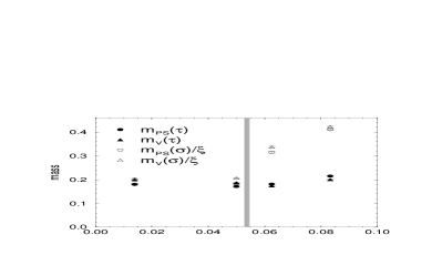
Figure 5: Temperature dependence of the pole and the screening masses for $\kappa_{\sigma}=0.081$(top figure), and at the chiral limit (bottom). The vertical gray lines roughly represent the critical temperature.

Both pole and screening masses are extrapolated to the chiral limit from the 3 quark masses analyzed. The extrapolation is done using $\kappa$ of eq. (5). Below the critical temperature the pion masses squared $m_{ps}^{2}$ are extrapolated, in all other cases, the masses themselves are extrapolated linearly in $1/\kappa$. The extrapolation of the pole masses at $T=0$ gives the critical value $\kappa_{c}=0.17138(20)$ and $a_{\sigma}^{-1}=1.18$ GeV from the $\rho$ mass using $\xi=5.3$. The result of the screening mass extrapolation is almost the same – see Fig 6. The large difference between $a_{\sigma}^{-1}(\rho)$ and $a_{\sigma}^{-1}$ from the heavy quark potential (see the table) indicates significant discretization effects for our lattices as expected. The results are summarized in the second plot in Fig. 5. We find large differences between the pole and the screening masses above $T_{c}$ both at finite quark masses and in the chiral limit. We should like to point out that a similar behavior is obtained in an effective model approach with NJL Lagrangian [8].

Figure 6: Chiral extrapolation of the pion screening masses at various $T$.

6 Topological properties

To determine the topological properties of the configurations we use improved cooling – see [9]. Unlike usual cooling with Wilson action this method preserves instantons at scales larger than a certain dislocation threshold $\rho_{0}$. For anisotropic lattices the improved action is modified accordingly ensuring isotropic distributions for the sizes and distances of instantons at $T=0$. From earlier investigations we expect a scale of about 0.4 - 0.7 fm to be relevant for the topology of $SU(3)$. With a dislocation threshold $\rho_{0}\sim 2a\simeq 0.5$ fm the lattices used here are too coarse for a detailed analysis. Nevertheless we obtain reasonable data for the susceptibility in agreement with Witten-Veneziano formula below $T_{c}$ and dropping to zero at high temperature, in agreement with other analysis on finer lattices. An interesting quantity is the ratio $R(k)=Q_{t}^{2}(kV)/Q_{s}^{2}(kV)$ between the charge in subvolumes $kV$ obtained by slicing the lattice in either a spatial or a temporal direction. The temperature effect shows up in an anisotropy between temporal and spatial slicing which sets in when the dominant sizes begin to feel the limited temporal extension. Just below $T_{c}$ $R(1/2)$ in the charge zero sector is about 0.7, while above $T_{c}$ (where all configurations have $Q=0$) $R(1/2)$ grows fast to about 3. This behavior is compatible with a random distribution of instantons of rather large sizes below $T_{c}$ and a tendency to form pairs above $T_{c}$. Generally, there seems to be a qualitative difference between the instanton population below and above $T_{c}$: at similar densities of pairs the instantons of the low temperature are reasonably well fitted by the ’t Hooft ansatz, while at high temperature we seem to deal with topological charge fluctuations which hardly can accommodate the continuum picture of instantons. A more detailed account of these features will be given elsewhere.

7 Conclusions and outlook

The present analysis has produced results about the temperature effects on the vacuum and hadronic properties in quenched QCD which are consistent with the following picture: below $T_{c}$ the changes are small and gradual while above $T_{c}$ the changes increase strongly (but not abruptly) with the temperature; at temperatures of about $1.5T_{c}$ the mesons have become unstable and are strongly interacting with a significant quark-gluon plasma component; the changes in the vacuum structure follow a similar pattern and there is indication of close range opposite charge correlation (although there are no dynamical fermions).

This picture needs to be further tested in order to remove the uncertainties still affecting the present analysis. This concerns particularly the question of an unambiguous definition of the hadron states at high temperature. In the further developments we shall also try to extract directly information about the spectral function of the hadronic correlators [10], use larger lattices such that we can both have larger physical distances and a smaller lattice spacing (in spatial directions) for more refined studies of the topology, and aim, of course, to an improved statistics.

The calculations have been done on AP1000 at Fujitsu Parallel Computing Research Facilities and Paragon at INSAM, Hiroshima Univ.

References

- [1] N.P. Landsman and Ch.G. van Weert, Phys. Rep. 145 (1987) 141.
- [2] QCD-TARO: M. Fujisaki et al., in Multi-scale Phenomena and their Simulation, F. Karsch, B. Monien and H. Satz eds., World Scientific (Singapore 1997) 208.
- [3] S. Sakai, A. Nakamura and T. Saito, these proceedings.
- [4] QCD-TARO: M. Fujisaki et al., Nucl. Phys. B (Proc.Suppl.) 53 (1997) 426.
- [5] T. Hashimoto, A. Nakamura and I.-O. Stamatescu, Nucl. Phys. B400 (1993) 267.
- [6] J. Kupsch and I.-O. Stamatescu, work in progress.
- [7] QCD-TARO: M. Fujisaki et al., in Confinement 95, H. Toki et al eds., World Scientific (Singapore 1995) 129.
- [8] T. Hatsuda and T. Kunihiro, Phys. Rep. 247 (1994) 221.
- [9] Ph. de Forcrand, M. García Pérez and I.-O. Stamatescu, Nucl. Phys. B499 (1997) 409.
- [10] QCD-TARO: Ph. de Forcrand et al., Nucl. Phys. B (Proc.Suppl.) 63 (1998) 460.