DESY 98–124
HUB–EP–98/46
FUB-HEP/3-98
TPR-98-29
September 1998
Nucleon form factors and $O(a)$ Improvement

Abstract

Nucleon form factors have been extensively studied both experimentally and theoretically for many years. We report here on new results of a high statistics quenched lattice QCD calculation of vector and axial-vector nucleon form factors at low momentum transfer within the Symanzik improvement programme. The simulations are performed at three $\kappa$ and three $\beta$ values allowing first an extrapolation to the chiral limit and then an extrapolation in the lattice spacing to the continuum limit. The computations are all fully non-perturbative. A comparison with experimental results is made.

1 INTRODUCTION

For many years experiments have been performed with electron–nucleon scattering to obtain information about the structure of the nucleon. Form factors are defined from the general decomposition of the proton, $p$ (or neutron, $n$) matrix element ($q=p-p^{\prime}$):

$$\langle\vec{p},\vec{s}|\widehat{\cal V}^{\mbox{\small$\frac{2}{3}$}u-\mbox{\small$\frac{1}{3}$}d}_{\mu}(\vec{q})|\vec{p}^{\prime},\vec{s}^{\prime}\rangle=$$

$$\overline{u}(\vec{p},\vec{s})\left[\gamma_{\mu}F^{p}_{1}+\sigma_{\mu\nu}{q_{\nu}\over 2m}F^{p}_{2}\right]u(\vec{p}^{\prime},\vec{s}^{\prime}).$$

We have $F_{1}(0)=1$ as ${\cal V}$ is a conserved current, while $F_{2}(0)=\mu-1$ measures the anomalous magnetic moment (in magnetons). Usually we define the Sachs form factors:

$$G_{e}(-q^{2}) = F_{1}(-q^{2})+{-q^{2}\over(2m)^{2}}F_{2}(-q^{2}),$$

$$G_{m}(-q^{2}) = F_{1}(-q^{2})+F_{2}(-q^{2}).$$

Experiments lead to phenomenological dipole fits:

$$G_{e}^{p}(-q^{2}) \sim {G_{m}^{p}(-q^{2})\over\mu^{p}}\quad\sim\quad{G_{m}^{n}(-q^{2})\over\mu^{n}}$$

$$= 1/\left(1+\left(-q^{2}/m_{V}^{2}\right)\right)^{2},$$

$$G_{e}^{n}(-q^{2}) \sim 0,$$

with $m_{V}\sim 0.82$ GeV, $\mu^{p}\sim 2.79$, $\mu^{n}\sim-1.91$.

Neutrino–neutron scattering, $n\nu_{\mu}\to p\mu^{-}$, gives from the charged weak current the axial form factor $g_{A}(-q^{2})$. In addition $g_{A}(0)$ is also accurately obtained from $\beta$-decay, $n\to pe^{-}\overline{\nu}$. Upon using current algebra this form factor can be related to the matrix element:

$$\langle\vec{p},\vec{s}|\widehat{\cal A}^{u-d}_{\mu}(\vec{q})|\vec{p}^{\prime},\vec{s}^{\prime}\rangle=$$

$$\overline{u}(\vec{p},\vec{s})\left[\gamma_{\mu}\gamma_{5}g_{A}+i\gamma_{5}{q_{\mu}\over 2m}h_{A}\right]u(\vec{p}^{\prime},\vec{s}^{\prime}).$$

The phenomenological fits are:

$$g_{A}(q^{2})=g_{A}(0)/\left(1+\left(-q^{2}/m_{A}^{2}\right)\right)^{2},$$

with $g_{A}(0)=1.26$, $m_{A}\sim 1.00$ GeV.

2 THE LATTICE METHOD

Quenched configurations have been generated at $\beta=6.0$ ($O(500)$, $16^{3}\times 32$ lattice) $\beta=6.2$ ($O(300)$, $24^{3}\times 48$ lattice) and $\beta=6.4$ ($O(100)$, $32^{3}\times 48$ lattice), [1]. By forming the ratio of three-to-two point functions, [2]:

$$R_{\alpha\beta}(t,\tau;\vec{p},\vec{q})={\langle N_{\alpha}(t;\vec{p}){\cal O}(\tau;\vec{q})\overline{N}_{\beta}(0;\vec{p}^{\prime})\rangle\over\langle N(t;\vec{p})\overline{N}(0;\vec{p})\rangle}\times$$

$$\left[{\langle N(\tau;\vec{p})\overline{N}(0;\vec{p})\rangle\langle N(t;\vec{p})\overline{N}(0;\vec{p})\rangle\langle N(t-\tau;\vec{p}^{\prime})\overline{N}(0;\vec{p}^{\prime})\rangle\over\langle N(\tau;\vec{p}^{\prime})\overline{N}(0;\vec{p}^{\prime})\rangle\langle N(t;\vec{p}^{\prime})\overline{N}(0;\vec{p}^{\prime})\rangle\langle N(t-\tau;\vec{p})\overline{N}(0;\vec{p})\rangle}\right]^{\mbox{\small$\frac{1}{2}$}}$$

$$\propto\langle N_{\alpha}(\vec{p})|\widehat{\cal O}(\vec{q})|N_{\beta}(\vec{p}^{\prime})\rangle,$$

the appropriate matrix elements can be found. (Only the quark line connected part of the $3$-point function is considered.) For each $\beta$ we chose three $\kappa$ values and a variety of $3$-momenta: $\vec{p}=2\pi/N_{s}\{$ $(0,0,0)$, $(1,0,0)$ $\}$, $\vec{q}=2\pi/N_{s}\{$ $(0,0,0)$, $(0,1,0)$, $(0,2,0)$, $(1,0,0)$, $(2,0,0)$, $(1,1,0)$, $(1,1,1)$, $(0,0,1)$ $\}$ together with the nucleon either unpolarised or polarised in the $y$ direction. (Some combinations were too noisy to be used though.) After sorting the matrix elements into $q^{2}$ classes (defined by $q^{2}$ in the chiral limit), $4$-parameter fits are made assuming that the form factors are linear in the bare quark mass $am_{q}$. $O(a)$ improved Symanzik operators are used:

$${\cal V}_{\mu}^{R} = Z_{V}(1+b_{V}am_{q})\times$$

$$\quad\left[\bar{\psi}\gamma_{\mu}\psi+\mbox{\small$\frac{1}{2}$}ic_{V}a\partial_{\lambda}(\bar{\psi}\sigma_{\mu\lambda}\psi)\right],$$

$${\cal A}_{\mu}^{R} = Z_{A}(1+b_{A}am_{q})\times$$

$$\quad\left[\bar{\psi}\gamma_{\mu}\gamma_{5}\psi+\mbox{\small$\frac{1}{2}$}c_{A}a\partial_{\mu}(\bar{\psi}\gamma_{5}\psi)\right],$$

where $Z_{V}$, $Z_{A}$, $b_{V}$, $c_{V}$, $c_{A}$ (and $c_{sw}$) have been non-perturbatively calculated by the Alpha collaboration, [3]. All matrix elements thus are correct to $O(a^{2})$. We can check $Z_{V}$ as ${\cal V}_{\mu}$ is a conserved current (ie $F_{1}(0)=1$). In Fig. 1

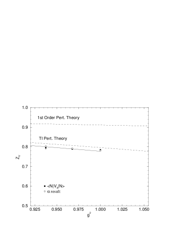
Figure 1: $Z_{V}$ for improved fermions. Shown is the lowest order perturbation result together with a tadpole-improved version (as given in [4]). The non-perturbative determinations are shown as open circles, [3], and filled squares, this work.

we show a comparison of the two determinations of $Z_{V}$. Very good agreement is seen. This is not the case when Wilson fermions are used (see ref. [5]). Finally we note that although we have included the improvement terms in our operators, numerically they seem to have little influence on the value of the matrix element.

3 RESULTS

In Fig. 2

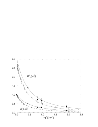
Figure 2: The proton form-factors $G^{p}_{e}(-q^{2})$ and $G^{p}_{m}(-q^{2})$ against $-q^{2}$ showing experimental results (open circles, taken from ref. [6]) and lattice results (filled circles, $\beta=6.2$ only). The string tension is used to fix the scale as in [4]. All fits are dipole fits.

we show $G^{p}_{e}(-q^{2})$ and $G^{p}_{m}(-q^{2})$ for $\beta=6.2$ together with experimental results (also plotting the other $\beta$ values tends to clutter the picture). Making dipole fits gives Fig. 3 for the continuum extrapolation.

Figure 3: $m_{V}$ from $\beta=6.0$, $6.2$, $6.4$ against $a^{2}$. The phenomenological value is also given at $a^{2}=0$.

There seems to be little inclination for $m_{V}$ to approach the experimental result. (A roughly similar result is obtained from $G^{p}_{m}$, although due to larger error bars the results are more compatible.)

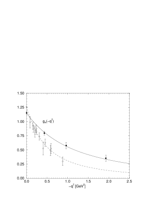
Figure 4: $g_{A}(-q^{2})$ against $-q^{2}$, notation as in Fig. 2.

Figure 5: The continuum extrapolation of $m_{A}$.

For the axial current we find the results in Figs. 4, 5. The form factor fall-off is again too soft as $m_{A}$ is too large. However the important $g_{A}(0)$ is faring better, see Fig. 6.

Figure 6: The continuum extrapolation of $g_{A}(0)$.

4 CONCLUSIONS

We have performed simulations at three $\beta$ values so that an attempt can be made to take the continuum extrapolation, $a\to 0$. While the lattice dipole masses seem to be too large, $g_{A}(0)$ is in reasonable agreement with the experimental result. The mass discrepancies may be due to a quenching effect, although only similar simulations using dynamical fermions will be able to answer this.

References

- [1] D. Pleiter, this conference.
- [2] G. Martinelli et al., Nucl. Phys. B316 (1989) 355; W. Wilcox et al., Phys. Rev. D46 (1992) 1109, hep-lat/9205015 ; K. F. Liu et al., Phys. Rev. D49 (1994) 4755, hep-lat/9305025.
- [3] M. Lüscher et al., Nucl. Phys. B491 (1997) 323, hep-lat/9609035; Nucl. Phys. B491 (1997) 344, hep-lat/9611015; M. Guagnelli et al., Nucl. Phys. (Proc Suppl) 63 (1998) 886, hep-lat/9709088.
- [4] M. Göckeler et al., Phys. Rev. D57 (1998) 5562, hep-lat/9707021.
- [5] S. Capitani et al., Ahrenshoop Symposium, Buckow, Germany (Wiley-VCH 1998), hep-lat/9801034.
- [6] C. V. Christov et al., Prog. Part. Nucl. Phys. 37 (1996), hep-ph/9604441.