Numerical Studies of the Double Scaling Limit
in a Large $N$ Reduced Model

Abstract

We study the two-dimensional Eguchi-Kawai model as a toy model of the IIB matrix model, which has been recently proposed as a nonperturbative definition of the type IIB superstring theory. While the planar limit of the model is known to reproduce the two-dimensional Yang-Mills theory, we find through Monte Carlo simulation that the model allows a different large $N$ limit, which can be considered as the double scaling limit in matrix models.

1 INTRODUCTION

Large $N$ (partially) reduced models (See Ref. [1] for a review.) revived recently in the context of string theory [2, 3]. The IIB matrix model [3] is a matrix model, which can be obtained by the dimensional reduction of the 10D large $N$ super Yang-Mills theory to 0D (a point). It is conjectured to provide a nonperturbative definition of type IIB superstring theory in the double scaling limit. One of the interesting features of this model is that all the target-space coordinates come out as the eigenvalues of the matrices.

Nonperturbative studies of the bosonic string theory in less than one dimension were successfully done through the double scaling limit of the matrix model [4] some time ago. On the other hand, large $N$ reduced models have been studied so far exclusively in the planar limit, in which the models are equivalent to the field theory before being reduced. Whether a large $N$ reduced model allows any sensible double scaling limit, which enables an interpretation as a string theory, is itself a nontrivial question.

In this article, we report on our studies [5] of the two-dimensional Eguchi-Kawai (EK) model [6], as a toy model of the IIB matrix model. The model is nothing but an SU($N$) lattice gauge theory on a $1\times 1$ lattice with a periodic boundary condition and it is equivalent to an SU($N$) lattice gauge theory on an infinite lattice in the planar limit. We perform a Monte Carlo simulation of the model and find that the model indeed allows a different large $N$ limit, which can be considered as the double scaling limit in matrix models.

2 EK MODEL AND PLANAR LIMIT

The EK model is defined by the following action [6].

$$S_{EK}=-N\beta\sum_{\mu\neq\nu=1}^{D}\mbox{tr}\{U_{\mu}U_{\nu}U^{{\dagger}}_{\mu}U^{{\dagger}}_{\nu}\}.$$ (1)

This model has a U(1)^D symmetry.

$$U_{\mu}\to e^{i\theta_{\mu}}U_{\mu}.$$ (2)

In Ref. [6], it has been shown that if the U(1)^D symmetry is not spontaneously broken, the model is equivalent to an SU($N$) lattice gauge theory on an infinite lattice in the large $N$ limit, where the coupling constant $\beta$ in the action (1) is kept fixed. This limit is referred to as the planar limit, since in this limit Feynman diagrams with planar topology dominate. The observable which corresponds to the Wilson loop in the ordinary lattice gauge theory can be defined by

$$w(C)=\frac{1}{N}\mbox{tr}\left\{U_{\alpha}U_{\beta}U_{\gamma}\cdots U_{\lambda}\right\},$$ (3)

where only the direction of the links on which the link variables sit is maintained.

In two dimensions, the U(1)² symmetry is not spontaneously broken, and therefore the EK model is equivalent to the lattice gauge theory in the planer limit in the above sense. The two-dimensional lattice gauge theory is solvable [7] in the planar limit and indeed the exact results obtained there have been reproduced by the EK model in the planar limit [6].

The planar result for the expectation value of rectangular Wilson loops is given by [7]

$$\langle W(I\times J)\rangle=\exp\left(-\kappa(\beta)IJ\right),$$ (4)

where

$$\kappa(\beta)=\left\{\begin{array}[]{ll}-\log\beta&\;\;\;\mbox{for}\;\;\;\beta\leq\frac{1}{2}\\ -\log\left(1-\frac{1}{4\beta}\right)&\;\;\;\mbox{for}\;\;\;\beta\geq\frac{1}{2}.\end{array}\right.$$ (5)

This result shows that the rectangular Wilson loops obey an area law exactly for all $\beta$. From this result, one can figure out how to fine-tune the coupling constant $\beta$ as a function of the lattice spacing $a$ when one takes the continuum limit $a\rightarrow 0$. Since the physical area is given by $S=a^{2}IJ$, we have to fine-tune $\beta$ so that $\kappa(\beta)/a^{2}$ is kept fixed. We therefore take

$$a=\sqrt{\kappa(\beta)}$$ (6)

in the following. Since $\kappa(\beta)$ is given by eq. (5), we have to send $\beta$ to infinity as we take the $a\rightarrow 0$ limit.

In Fig. 1 we plot the expectation value of square Wilson loops in the EK model against the physical area $S=(aI)^{2}$ for $\beta=4.0$ with $N=16,32,64$ and $128$. One can see that the data points approach the planar result from above monotonically as we increase $N$. This is not the case when the boundary condition is twisted [5].

Figure 1: The expectation value of $w(I\times I)$ in the EK model for $\beta=4.0$ is plotted against the physical area $S=(aI)^{2}$. The straight solid line represents the planar result by Gross-Witten.

3 DOUBLE SCALING LIMIT

We consider the EK model as a toy model of the IIB matrix model. Just as in Ref. [3], we make the T-duality transformation, when we interpret the EK model as a string theory. Since the EK model can be considered to be defined on a unit cell of size $a$ with a periodic boundary condition, it can be considered, after the T-duality transformation, as a string theory in the two-dimensional space time compactified on a torus of size $1/a$.

The observables we consider in this section are the Wilson loops

$$\mbox{tr}\left\{U_{\alpha}U_{\beta}U_{\gamma}\cdots U_{\lambda}\right\},$$ (7)

where the suffix $\alpha,\beta,\cdots,\lambda$ runs over $\pm 1$,$\pm 2$ and $U_{-\alpha}$ ($\alpha>0$) is defined by $U_{-\alpha}=U_{\alpha}^{\dagger}$. The winding number of the Wilson loop is given by $n_{\mu}=\hat{\alpha}_{\mu}+\hat{\beta}_{\mu}+\cdots+\hat{\lambda}_{\mu}$, where $\hat{\alpha}_{\mu}$ denotes a unit vector in the $\alpha$ direction. Note that the observables (3) considered in the previous section can be viewed as the Wilson loops in the EK model with $n_{\mu}=0$, while in this section we consider those with $n_{\mu}\neq 0$ as well. After the T-duality transformation, the winding of the Wilson loops represents the momentum distribution of the string in the two-dimensional space time.

In what follows, we consider

$$O^{(n)}_{\alpha\beta}(L) = \mbox{tr}(U_{\alpha}^{L}U_{\beta}^{L}U_{-\alpha}^{L}U_{-\beta}^{L})$$

$$O^{(w)}_{\alpha}(L) = \mbox{tr}(U_{\alpha}^{L}),$$ (8)

which give typical Wilson loops in the non-winding sector and the winding sector respectively. When we take the $a\rightarrow 0$ limit, we have to send $L$ to the infinity by fixing $aL$.

Let us examine the one-point function of Wilson loops in the non-winding sector, namely $G_{1}^{(n)}(L)=\langle O^{(n)}_{12}(L)\rangle$. The observable $\langle w(L\times L)\rangle$ considered in the previous section is nothing but $N^{-1}G_{1}^{(n)}(L)$. We have seen in Fig. 1 how the data for $N^{-1}G_{1}^{(n)}(L)$ approach the planar limit when we increase $N$ with fixed $\beta$. We find that $N^{-1}G_{1}^{(n)}(L)$ scales in the large $N$ limit by fixing $\beta/N$. In Fig. 2 we show the data for $\beta/N=1.0/32$ and $\beta/N=1.5/32$. $N$ is taken to be $32,48,64,96$ and $128$.

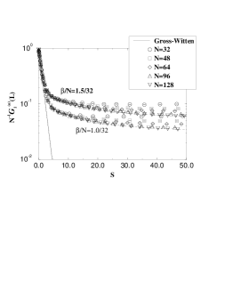
Figure 2: The one-point function of the Wilson loops in the non-winding sector $N^{-1}G_{1}^{(n)}(L)$ in the EK model is plotted against $S=(aL)^{2}$ for the sets of $\beta$ and $N$ with $\beta/N$ fixed to $1.0/32$ and $1.5/32$. The straight solid line represents the planar result by Gross-Witten. The dashed lines, which connect the data for $N=128$, are drawn to guide the eye.

From this observation, it is natural to expect that the double scaling limit of the EK model can be taken by fixing $\beta/N$, which corresponds to the string coupling constant $g_{str}$. The planar limit corresponds to $g_{str}=0$. We have also observed [5] a clear scaling behavior for other Green functions; e.g.,

$$G_{2}^{(w)}(L)=\langle O_{\mu}^{(w)}(L)O_{-\mu}^{(w)}(L)\rangle.$$ (9)

4 CONCLUSION AND DISCUSSION

To summarize, our numerical results strongly suggest the existence of a double scaling limit in the 2D EK model. In this limit, the density of eigenvalues is constant on a physical scale. As we mentioned above, the extent of space time is given by $R=1/a$. Since we have $N$ eigenvalues distributed in a two-dimensional space time with this extent, the average density is given by $N/R^{2}=Na^{2}$, which is constant in the double scaling limit. This fact is natural from a string theoretical point of view, since it means that there are only finite dynamical degrees of freedom on average in a finite region of space time.

The fact that a sensible double scaling limit can be taken for a large $N$ reduced model is itself encouraging for the study of a nonperturbative formulation of superstring theory through the IIB matrix model. We hope to report on numerical studies of the IIB matrix model in future publications.

References

- [1] S.R. Das, Rev. Mod. Phys. 59 (1987) 235.
- [2] T. Banks, W. Fischler, S.H. Shenker and L.Susskind, Phys. Rev. D55 (1997) 5112.
- [3] N. Ishibashi, H. Kawai, Y. Kitazawa and A. Tsuchiya, Nucl. Phys. B498 (1997) 467.
-
[4]
E. Brézin and V.A. Kazakov,
Phys. Lett. B236 (1990) 144.
M.R. Douglas and S.H. Shenker, Nucl. Phys. B335 (1990) 635.
D.J. Gross and A.A. Migdal, Phys. Rev. Lett. 64 (1990) 127. - [5] T. Nakajima and J. Nishimura, Nucl. Phys. B528 (1998) 355.
- [6] T. Eguchi and H. Kawai, Phys. Rev. Lett. 48 (1982) 1063.
- [7] D.J. Gross and E. Witten, Phys. Rev. D21 (1980) 446.