HLRZ-1998-56
WUB-98/32
Multicanonical Hybrid Monte Carlo:
Boosting Simulations of Compact QED

Abstract

We demonstrate that substantial progress can be achieved in the study of the phase structure of 4-dimensional compact QED by a joint use of hybrid Monte Carlo and multicanonical algorithms, through an efficient parallel implementation. This is borne out by the observation of considerable speedup of tunnelling between the metastable states, close to the phase transition, on the Wilson line. We estimate that the creation of adequate samples (with order 100 flip-flops) becomes a matter of half a year’s runtime at 2 Gflops sustained performance for lattices of size up to $24^{4}$.

1 Introduction

It appears exceedingly intriguing to define variants of QED by studying vacuum states other than the usual perturbative vacuum. Lattice techniques have the potential power to deal with this situation, whenever they provide us with phase transition points of second and higher orders.

It is embarrassing that lattice simulations of compact QED still have not succeeded to clarify the order of the phase transition near $\beta=1$, the existence of which was established in the classical paper of Guth [1]. This is mainly due to the failure of standard updating algorithms, like metropolis, heatbath or metropolis with reflections [2, 3, 4, 5], to move the system at sufficient rate between the observed metastable states near its phase transition. The tunneling rates decrease exponentially in $L^{3}$ and exclude the use of lattices large enough to make contact with the thermodynamic limit by finite size scaling techniques (FSS) [6].

In this paper, we propose to make use of the multicanonical (MUCA) algorithm [7] within the hybrid Monte Carlo (HMC) updating scheme [8] in order to boost the tunneling rates. Since both algorithms are inherently of global nature, their combination will facilitate the parallelization of MUCA which could not be achieved otherwise.

In the early days of simulations on the hyper-torus, the U(1) phase transition was claimed to be second-order [9, 10, 11, 12], however, with increasing lattice sizes, metastabilities and double peak action distributions became manifest, strongly hinting at its first-order character [13, 14, 15]. This picture is in accord with various renormalization group studies [16, 17].

However, the latent heat is found to decrease with the lattice size and the critical exponent $\nu$ is neither 0.25 (first order) nor $0.5$ (trivially second-order) [18]. These facts allow for two possible propositions:

1. the double peak structure is a finite size effect and might vanish in the thermodynamic limit, leading to the signature of a second-order phase transition;

2. the phase transition is weakly first-order, i. e., the correlation length $\xi$ is finite, but large in terms of the available lattice extent $L$; this would fake, on small lattices, the signature of a second-order transition, and a stabilized value of the latent heat would only become visible in the thermodynamic limit $L>\xi$ .

In search for a lattice formulation of QED with a second-order transition point, the action was generalized to include a piece in the adjoint representation with coupling $\gamma$ [19], in the expectation that the phase transition would be driven towards second-order, at sufficiently small negative values of $\gamma$. However, simulations on the hyper-torus, up to $\gamma=-0.4$, revealed the reappearance of a double peak on large enough lattices [20, 21]. Thus, the hypothesis of a second-order phase transition at some finite negative value of $\gamma$ [22, 23, 24] is again doubted; furthermore, renormalization group investigations indicated that the second-order phase transition is located at $\gamma\rightarrow-\infty$ [17].

Ref. [25] has speculated that the mechanism behind the lattice heuristics of metastabilities is driven by monopole loops that wrap around the hyper-torus. According to this scenario, the inefficiency of local updating algorithms to create and annihilate such monopole constellations causes their slowing down, in agreement with the earlier proposition (1). Results were presented in support of this view by switching to spherical lattices with trivial homotopy group where such wrapping loops are no more topologically stabilized [26, 27, 28, 29]. But on spherical lattices equivalent to $L=26$ at $\gamma=-0.2$, double peak structures have recently been reported to reappear [20, 21], corroborating earlier observations with periodic boundary conditions at $\gamma=0$: the suppression of monopole loop penetration through the lattice surface turned out to be incapable of preventing the incriminated double peak signal to show up on large lattices, to say $L=32$ [30, 31, 32].

It appears that a clarification of the situation on the Wilson line is mandatory for further progress in the understanding of compact lattice QED! This challenge requires the design of more powerful updating algorithms. A promising method is based on simulated tempering [33, 34, 35], enlarging the Lagrangian by a monopole term whose coupling is treated as an additional dynamical variable. Multi-scale update schemes in principle can alleviate critical slowing down (CSD) which is associated with the increase of the correlation length $\xi$ (as measured in a non-mixed phase) near the critical coupling, $\beta_{c}$ [36]. However, the exponential supercritical slowing down (SCSD) which is a consequence of the surface tension at first-order phase transitions cannot be overcome by such type of scale-adapted methods. In that instance, one expects the autocorrelation times to grow exponentially with the system size due to the occurrence of two 3-dimensional interfaces, leading to

$$\tau_{\mbox{\tiny SCSD}}\propto\exp\left(2\sigma L^{3}\right).$$ (1)

Torrie and Valleau [37, 38, 39, 40] have shown how to generate arbitrary “non-physical” sampling distributions. Their method, termed “umbrella sampling”, has been introduced to span large regions of phase diagrams. The method is capable to improve the efficiency of stochastic sampling for situations when dynamically nearly disconnected parts of phase space occur by biassing the system to frequent the dynamically depleted, connecting regions of configuration space. They interpreted their method as sampling “a whole range of temperatures” [37].

In recent years the idea of “umbrella sampling” has been popularized and extensively applied under the name “multi-canonical algorithm” (MUCA) by Berg and Neuhaus [7, 41, 42, 43, 44] to the simulation of a variety of systems exhibiting first-order phase transitions [45, 46, 47, 48, 49, 50]. In this procedure, the biassing weight $w(S)$ of a configuration with action $S$ is dynamically adjusted (bootstrapped) such as to achieve a near-constant overall frequency distribution over a wide range of $S$ within a single simulation.

Obviously, MUCA in principle offers a powerful handle to deal with SCSD. It remains then a practical question whether one can indeed proceed to large lattices by boosting tunneling rates from the SCSD behaviour (eq. (1)) to the peak efficiency of local Monte Carlo methods (characterized by ${O}((L^{4})^{2})$ complexity). This leads us to the key point of this paper: it is a severe shortcoming of the multi-canonical algorithm that its implementation is seemingly restricted to sequential computers, as it requires knowledge of the global action, even during local updating. We will show that HMC is from the very outset able to implement MUCA in a parallel manner.

In sections 2.1 and 2.2, we will give a short review of the MUCA and the HMC algorithms. In section 2.3, we merge MUCA with HMC. From our ongoing simulation project of U(1) theory on the Wilson line [51], we determine the tunneling efficiency compared to the standard metropolis algorithm which in our case is complemented by three reflection steps. In section 3, we shall present our results for lattice sizes up to $16^{4}$ and predict the tunnelling rates for lattice sizes up to $24^{4}$, as would be required for a proper FSS.

2 Multicanonical Hybrid Monte Carlo

The hybrid Monte Carlo (HMC) algorithm [8, 52, 53] produces a global trial configuration by carrying out a molecular dynamics evolution of the field configuration very close to the surface of constant action. Subsequently, a Monte Carlo decision is imposed which is based on the global action difference $\Delta S$, being small enough to be frequently accepted. Within HMC, all degrees-of-freedom can be changed simultaneously and hence in parallel. This then provides the straightforward path to implement MUCA as part of HMC on parallel machines: one just uses the values of the global action, as provided by HMC, to compute the bias function $w(S)$ for the MUCA algorithm.

2.1 Multicanonical Algorithm

“Canonical” Monte Carlo generates a sample of field configurations, $\left\{\phi\right\}$, within a Markov process, according to the Boltzmann weight,

$$P_{\beta}(S)=\frac{1}{Z_{\mbox{\tiny can}}}e^{-\beta S(\phi)},$$ (2)

which follows from maximizing the entropy with respect to all possible probability distributions $P[\phi]$. The partition function $Z$ normalizes the total probability to 1,

$$Z_{\beta}=\int[d\phi]\,e^{-\beta S[\phi]}.$$ (3)

$S$ is the action (the energy in the case of statistical mechanics) and $\beta$ the coupling (or inverse temperature $\frac{1}{kT}$).

The canonical action density which in general exhibits a double peak structure at a first-order phase transition, can be rewritten as

$$N_{\mbox{\tiny can}}(S,\beta)=\rho(S)\,e^{-\beta S},$$ (4)

with the spectral density $\rho(S)$ being independent of $\beta$. Usually, $\int N_{\mbox{\tiny can}}(S,\beta)\,dS$ is set to 1.

The multicanonical approach aims at generating a flat action density

$$N_{\mbox{\tiny MUCA}}(S,\beta)=\mbox{const., \hskip 14.22636pt for }S_{\mbox{\tiny min}}\leq S\leq S_{\mbox{\tiny max}},$$ (5)

in a range of $S$ that covers the double peaks at the first-order phase transition.

Therefore, instead of sampling canonically according to $e^{-\beta S}$, one modifies the sampling by a weight factor $W_{\mbox{\tiny MUCA}}$:

$$W_{\mbox{\tiny MUCA}}(S,\beta)=\left\{\begin{array}[]{rll}\frac{1}{\rho(S_{\mbox{\tiny min}})}&e^{\beta S_{\mbox{\tiny min}}}&\qquad\mbox{for}\;S<S_{\mbox{\tiny min}}\\ \frac{1}{\rho(S)}&e^{\beta S}&\qquad\mbox{for}\;S_{\mbox{\tiny min}}\leq S\leq S_{\mbox{\tiny max}}\\ \frac{1}{\rho(S_{\mbox{\tiny max}})}&e^{\beta S_{\mbox{\tiny max}}}&\qquad\mbox{for}\;S>S_{\mbox{\tiny max}},\\ \end{array}\right.$$ (6)

which is constant outside the relevant action range. Such ‘corrigez la fortune’ is equivalent to a net sampling according to the yet unknown probability distribution

$$w(S)=\frac{1}{\rho(S)},\qquad\mbox{for}\;S_{\mbox{\tiny min}}\leq S\leq S_{\mbox{\tiny max}}.$$ (7)

Since $W(S,\beta)$ is unknown at the begin of the simulation, it is instrumental for MUCA to follow Münchhausen and bootstrap from good guesstimates [43]. We shall do so by starting from an observed histogram of the canonical action density, $\hat{N}_{\mbox{\tiny can}}(S,\hat{\beta}_{c})$, see eq. (4), at the supposed location of the phase transition, $\hat{\beta}_{c}$. From the action density, we compute $\hat{W}_{\mbox{\tiny MUCA}}(S,\hat{\beta}_{c})$ according to eq. (6). The sampling then proceeds with the full MUCA weight,

$$\hat{P}_{\mbox{\tiny MUCA}}(S) \propto e^{-\hat{\beta}_{c}S}\hat{W}_{\mbox{\tiny MUCA}}(S,\hat{\beta}_{c})$$ (8)

$$\propto e^{-\big{(}\hat{\beta}_{c}+\hat{\beta}(S)\big{)}S-\hat{\alpha}(S)}.$$

This latter formulation can be interpreted as a simulation proceeding at varying couplings (temperatures), hence the naming ‘multicanonical’.

In order to compute expectation values of observables $\cal O$, one has to reweight the resulting action density at the end of the day by the factor $\hat{W}_{\mbox{\tiny MUCA}}(S,\hat{\beta}_{c})$, which reconstitutes the proper canonical density:

$$\langle\hat{\cal O}_{\hat{\beta}_{c}}\rangle=\frac{\sum_{i}{\cal O}^{i}_{\hat{\beta}_{c}}\,\frac{1}{\hat{W}_{\mbox{\tiny MUCA}}(S_{i},\hat{\beta}_{c})}}{\sum_{i}\frac{1}{\hat{W}_{\mbox{\tiny MUCA}}(S_{i},\hat{\beta}_{c})}}.$$ (9)

Additionally, $\langle\hat{\cal O}_{\hat{\beta}_{c}}\rangle$ simulated at $\hat{\beta}_{c}$ can be reweighted to any desired $\beta$ (following [55]), given that the corresponding region of phase space has been covered by the MUCA simulation. We emphasize that eq. (9) is only useful complemented by a proper error analysis. The canonical error computed from the multicanonical ensemble has been elaborated in Ref. [56].

Note that there are many possible choices for the form of the multicanonical weight. Just for technical reasons we require it to be continuous in $S$. One can either guess an analytic function, or choose a polygonal approximation such as given in eq. (8). In this case, the multicanonical weight is expressed in terms of the functions $\hat{\beta}(S)$ and $\hat{\alpha}(S)$ which are actually characteristic functions of the bins. $\hat{\beta}(S)$ can be considered as an effective temperature [37].

The computation of the weights requires the knowledge of the global and not just the local change in action for each single update step. For this reason, even for a local action, one cannot perform local updating moves in parallel, such as the well-known checkerboard pattern. As a consequence, MUCA is not parallelizable for local update algorithms. For remedy, we propose here to go global and utilize the HMC updating procedure.

2.2 Hybrid Monte Carlo

The HMC consists of two parts: the hybrid molecular dynamics algorithm (HMD) evolves the degrees of freedom by means of molecular dynamics (MD) which is followed by a global Metropolis decision to render the algorithm exact.

In addition to the gauge fields $\phi_{\mu}(x)$ one introduces a set of statistically independent canonical momenta $\pi_{\mu}(x)$, chosen at random according to a Gaussian distribution $\exp(-\frac{\pi^{2}}{2})$. The action $S[\phi]$ is extended to a guidance Hamiltonian

$${\cal H}[\phi,\pi]=\frac{1}{2}\sum_{\mu,x}\pi_{\mu}^{2}(x)+\beta S[\phi].$$ (10)

Starting with a configuration $(\phi,\pi)$ at MD time $t=0$, the system moves through phase space according to the equations of motion

$$\dot{\phi}_{\mu} = \frac{\partial{\cal H}}{\partial\pi_{\mu}}=\pi_{\mu},$$

$$\dot{\pi}_{\mu} = -\frac{\partial{\cal H}}{\partial\phi_{\mu}}=-\frac{\partial}{\partial\phi_{\mu}}[\beta S],$$ (11)

leading to a proposal configuration $(\phi^{\prime},\pi^{\prime})$ at time $t=\tau$. Finally this proposal is accepted in a global Metropolis step with probability

$$P_{acc}=\min\left(1,e^{-\Delta{\cal H}}\right),\quad\mbox{with}\ \Delta{\cal H}={\cal H}[\phi^{\prime},\pi^{\prime}]-{\cal H}[\phi,\pi].$$ (12)

The equations of motion are integrated numerically with finite step size $\Delta t$ along the trajectory from $t=0$ up to $t=N_{\mbox{\tiny md}}$. Using the leap-frog scheme as symplectic integrator the discretized version of eq. (2.2) reads:

$$\phi^{n+1} = \phi^{n}+\Delta t\cdot\pi^{n}-\frac{\Delta t^{2}}{2}\frac{\partial}{\partial\phi}\Big{(}\beta S[\phi^{n}]\Big{)}$$

$$\pi^{n+1} = \pi^{n}-\frac{\Delta t}{2}\frac{\partial}{\partial\phi}\Big{(}\beta S[\phi^{n}]\Big{)}-\frac{\Delta t}{2}\frac{\partial}{\partial\phi}\Big{(}\beta S[\phi^{n+1}]\Big{)}.$$ (13)

Here we have presented the scheme with both the momenta and the gauge fields defined at full time steps, $t=n\Delta t$.

To ensure that the Markov chain of gauge field configurations reaches a unique fixed point distribution $\exp(-S[\phi])$ one must require the updating procedure to fulfil detailed balance, which is guaranteed by the iterative map of eq. (2.2) $f:(\phi,\pi)\to(\phi^{\prime},\pi^{\prime})$ being

• time reversible: $f(\phi^{\prime},-\pi^{\prime})=(\phi,-\pi)$

• and measure preserving: $[d\phi^{\prime}][d\pi^{\prime}]=[d\phi][d\pi]$.

It is easy to prove that these two conditions also hold for the multicanonical action. Note that the guidance Hamiltonian, eq. (10), defining the MD may differ from the acceptance Hamiltonian in eq. (12), which produces the equilibrium distribution proper. In the following, we shall exploit this freedom to develop two variant mergers of MUCA and HMC.

2.3 Merging MUCA and HMC for Compact QED (MHMC)

We consider a multicanonical HMC for pure 4-dimensional $U(1)$ gauge theory with standard Wilson action defined as

$$S[\phi]=\sum_{x,\nu>\mu}\Big{[}1-\cos\big{(}\theta_{\mu\nu}(x)\big{)}\Big{]},$$ (14)

where

$$\theta_{\mu\nu}(x)=\phi_{\mu}(x)+\phi_{\nu}(x+\hat{\mu})-\phi_{\mu}(x+\hat{\nu})-\phi_{\nu}(x)$$

is the sum of link angles that contribute to one of six plaquettes interacting with the link angle $\phi_{\mu}(x)$.

Eq. 8 suggests to consider an effective action $\hat{S}$ including the “multicanonical potential” $V_{\mbox{\tiny MUCA}}$

$$\hat{S} = \hat{\beta}_{c}S+\hat{V}_{\mbox{\tiny MUCA}}(S,\hat{\beta}_{c}),$$ (15)

with

$$\hat{V}_{\mbox{\tiny MUCA}}(S,\hat{\beta}_{c}) = \log\Big{(}{\frac{1}{\hat{W}_{\mbox{\tiny MUCA}}(S,{\hat{\beta}}_{c})}}\Big{)}$$ (16)

$$= \hat{\beta}(S)\,S+\hat{\alpha}(S).$$

There are two natural options to proceed from here:

Method 1

performs molecular dynamics using the canonical guidance Hamiltonian

$${\cal H}_{md}=\frac{1}{2}\sum\pi^{2}+{\hat{\beta}_{c}}S,$$

with standard action $S$. The resulting gluonic force is given by

$$F(x) = \dot{\pi}_{\mu}(x)$$ (17)

$$= {\hat{\beta}}_{c}\sum_{\nu\not=\mu}\Big{[}\sin\theta_{\mu\nu}(x-{\hat{\nu}})-\sin\theta_{\mu\nu}(x)\Big{]}.$$

Method 2

makes use of the multicanonical potential as a driving term within the Hamiltonian,

$${\cal H}_{md}=\frac{1}{2}\sum\pi^{2}+\hat{S},$$

inducing an additional drift term

$$\dot{\pi}_{\mu}(x) = F(x)-\frac{\partial}{\partial\phi_{\mu}(x)}\hat{V}_{\mbox{\tiny MUCA}}\Big{(}S\big{[}\phi(x)\big{]},\hat{\beta}_{c}\Big{)}$$ (18)

$$= \Big{(}{\hat{\beta}_{c}}+{\hat{\beta}(S)}\Big{)}\sum_{\nu\not=\mu}\Big{[}\sin\theta_{\mu\nu}(x-{\hat{\nu}})-\sin\theta_{\mu\nu}(x)\Big{]},$$

with the effective $\hat{\beta}$ as defined in eq. (8).

For both options, the Hamiltonian governing the accept/reject decision, eq. (12), reads equally:

$${\cal H}_{\mbox{\tiny acc}}=\frac{1}{2}\sum\pi^{2}+\hat{S}.$$ (19)

The latter method is governed by the dynamics underlying the very two peak structure: as one can see from Fig. 5, $V_{\mbox{\tiny MUCA}}$ is repelling the system out of the hot (cold) phase towards the cold (hot) phase, thus increasing its mobility and enhancing flip-flop activity.

We comment that the implementation of method 2 requires the computation of the global action (to adjust the correct multicanonical weight, eq. (8)) at each integration step along the trajectory of molecular dynamics to guarantee reversibility. In the polygon approximation, this amounts to a determination of the effective coupling $\hat{\beta}$ at each time step in MD. Note that $\hat{\alpha}$ does not influence MD but enters into the global Metropolis decision, eq. (12). Method 1 is much simpler, running at fixed trial coupling $\hat{\beta}_{c}$ and avoiding the effort of computing $N_{\mbox{\tiny md}}-2$ global sums while travelling along the trajectories. It turned out that of both versions of MHMC, method 2 performs better than method 1, when autocorrelation and difference in computational effort are taken into account. Thus, we continue our analysis by investigation of method 2.

3 Results

In order to evaluate the efficiency of the MHMC and to set the stage for a proper extrapolation, we generated time series of the U(1) action on lattices of size $6^{4}$ up to $16^{4}$. The runs are summarized in Tab. 1. We applied method 2 as being the more promising one on real large lattices.

L	$\beta$	# sweeps(MRS)	# sweeps(MHMC)	$\Delta t$	$N_{md}$
6	1.001600	1.460.000	1.650.000	0.120	10
8	1.007370	1.320.000	1.430.000	0.093	13
10	1.009300	1.030.000	560.000	0.071	17
12	1.010150	680.000		0.060	20
	1.010143	1.790.000	1.160.000
14	1.010300	1.430.000		0.050	24
	1.010668	900.000	990.000
16	1.010800	1.210.000		0.045	26
	1.010753	750.000	760.000

Table 1: Total numbers of sweeps carried out both for MRS and MHMC at different lattice sizes $L$ and couplings $\beta$.

To arrive at an action density $N_{\mbox{\tiny MUCA}}(S,\beta)$ which is approximately flat in the desired region between the two peaks it is crucial to find a good estimate $\hat{N}_{\mbox{\tiny can}}(S,\hat{\beta}_{c})$ of the canonical action density. However, it becomes more and more delicate for large volumes to find the proper multicanonical weight, $\hat{P}_{\mbox{\tiny MUCA}}^{L}(S)$ (eq. (8)). Fig. 1 shows the evolution of the action density as the lattice size increases.

Figure 1: The canonical action densities, eq. (4), on $6^{4}$ up to $16^{4}$ lattices, reweighted to their respective $\hat{\beta}_{c}$ values, here defined via equal height of the histograms.

For lattices $<16^{4}$ it was sufficient to perform a short canonical run to generate an action density $\hat{N}_{\mbox{\tiny MUCA}}$ suitable to compute a proper weight factor $\hat{W}_{\mbox{\tiny MUCA}}$. On the $16^{4}$ system, however, the resulting multicanonical distribution becomes quite sensitive to the choice of the weight. Therefore, in the case of large lattices ($L\geq 16$) we cannot rely on canonical simulations to start with. Even if we perform $O(10^{6})$ sweeps using standard Metropolis update with 3 reflection steps, SCSD prevents a sufficiently accurate determination of the phase weight. Therefore, we install a recursive procedure: from a previous guess $\hat{N}_{\mbox{\tiny i}}(S,\hat{\beta}^{i}_{c})$ we go through MHMC and arrive at $\hat{N}_{\mbox{\tiny i+1}}(S,\hat{\beta}^{i+1}_{c})$. This computational scheme is initialized by a standard canonical “short run”. We found that one such learning cycle is sufficient. Fig. 2 illustrates the evolution of the multicanonical action density on the $16^{4}$ lattice.

Figure 2: Evolution of multicanonical action density. Starting from a canonical run a first MHMC simulation is performed (dashed line), and, based on this result, the final run (solid line) is carried out. Both curves are computed on the $16^{4}$ lattice at $\beta=1.010753$.

On larger volumes the determination of a good guess can be considerably boosted by a crank-up extrapolation that starts from smaller systems [43]. In Fig. 3, we display the quality of “flatness” of $\hat{N}_{\mbox{\tiny MUCA}}(S,\beta)$ achieved in our investigations for the various lattice sizes.

Figure 3: $\hat{N}_{\mbox{\tiny MUCA}}(S,\beta)$ at run-parameter $\beta$ as given in Tab. 2.

3.1 Tunneling Behaviour

With our estimate for $\hat{N}_{\mbox{\tiny MUCA}}^{16}(S)$ at $\beta=1.010753$, depicted in Fig. 2, we have generated the time history of the action per site, $s=S/6V$, as shown in the upper part of Fig. 4.

Figure 4: Time history of the $16^{4}$ system at $\beta=1.010753$ for MHMC (top) and MRS (bottom).

For reference, we have included the time history from the MRS algorithm on the same lattice. The figure demonstrates the success of MHMC: the method provides us with a gain factor in tunneling rate of about one order of magnitude on the $16^{4}$ lattice.

In order to quantify this achievement, we introduce the average flip time, $\tau_{\mbox{\tiny flip}}$, a quantity that is readily measurable. $\tau_{\mbox{\tiny flip}}$ is defined as follows: we histogram the time series of $s$ using $N$ bins, as illustrated in Fig. 5.

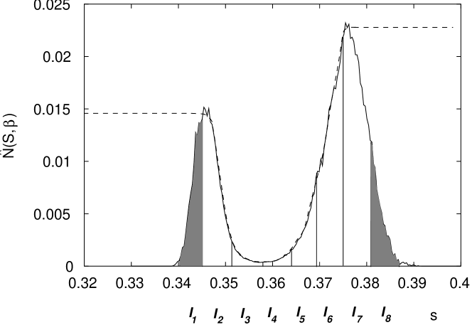
Figure 5: Action density of the $16^{4}$ system at ${\beta}=1.010753$ as a function of $s=\frac{S}{6V}$ from which $\hat{V}_{\mbox{\tiny MUCA}}$ is derived (the dashed line shows $\exp(\hat{V}_{\mbox{\tiny MUCA}})$). The subdivision of the support of the action density into 8 intervals is introduced in order to define $\tau_{\mbox{\tiny flip}}$.

A suitable number is $N=8$. The total binning range is adjusted such that $99.9$ % of the events are covered symmetrically by the 8 bins. A flip (flop) is given when the system travels from $I_{8}$ to $I_{1}$ (and vice versa). $\tau_{\mbox{\tiny flip}}$ is defined as the inverse number of the sum of flips and flops multiplied by the total number of trajectories. In Tab. 2, $\tau_{\mbox{\tiny flip}}$ is given for the various lattices. The error in $\tau_{\mbox{\tiny flip}}$ has been computed by a jackknife error analysis.

L	$\beta$	$\tau_{\mbox{\tiny flip}}^{\mbox{\tiny MRS}}$	$\tau_{\mbox{\tiny flip}}^{\mbox{\tiny MHMC}}$
6	1.001600	508(12)	650(20)
8	1.007370	1023(60)	1173(50)
10	1.009300	2474(117)	2006(84)
12	1.010143	5470(770)	3260(440)
14	1.010668	16400(3300)	5090(630)
16	1.010753	44800(9700)	6350(860)

Table 2: $\tau_{\mbox{\tiny flip}}$ for MRS and MHMC measured at the simulated $\beta$’s.

3.2 Scaling Behaviour

With the results for $\tau_{\mbox{\tiny flip}}$ on lattices up to $16^{4}$ we are in the position to estimate the scaling behaviour of MHMC in comparison to standard MRS updates. Fig. 6 shows $\tau_{\mbox{\tiny flip}}$ both for MHMC and MRS as a function of the lattice size $L$ at their respective $\beta$-values, as listed in Tab. 2.

Figure 6: Tunneling times for MRS (exponential fit) and MHMC (lower convex curve is power law, upper convex curve is exponential fit). The errors of the two exponential fits are depicted as dotted lines. The error of the power law fit, eq. (22), is not visible on this scale.

According to the expected exponential behaviour of $\tau_{\mbox{\tiny flip}}^{\mbox{\tiny MRS}}$ which, in the asymptotic regime $L\to\infty$, should be given by eq. (1), we perform a $\chi^{2}$-fit with the ansatz:

$$\tau_{\mbox{\tiny flip}}^{\mbox{\tiny MRS}}=a\ L^{b}\ e^{cL^{3}}.$$ (20)

It yields the following parameter values:

$$a = 11.9(3.7)$$

$$b = 2.01(18)$$

$$c = 6.7(8)\ 10^{-4},$$ (21)

with $\chi_{\mbox{\tiny per d.o.f.}}^{2}=0.897$. As a result, we find a clear exponential SCSD behaviour for the MRS algorihm.

On the other hand, for the tunneling times of the MHMC, we expect a monomial dependence in $L$:

$$\tau_{\mbox{\tiny flip}}^{\mbox{\tiny MHMC}}=p\ L^{q},$$ (22)

We obtain for the fit parameters:

$$p = 11.6(1.6)$$ (23)

$$q = 2.238(68).$$ (24)

The power law ansatz is well confirmed by the fit quality with $\chi_{\mbox{\tiny per d.o.f.}}^{2}=0.795$.

We also took the pessimistic ansatz and tried to detect a potentially exponential increase of $\tau_{\mbox{\tiny flip}}^{\mbox{\tiny MHMC}}$. The exponential fit gives $\chi_{\mbox{\tiny per d.o.f.}}^{2}=0.975$. As can be seen in Fig. 6, the exponential contribution remains suppressed in the extrapolation. A potentially dominating exponential behaviour for MHMC can only be detected in future MHMC simulations on larger lattices. In other words, parallel MHMC is capable to overcome SCSD in compact QED in practical simulations, at least up to lattices sizes $\approx 24^{4}$.

4 Cost Estimates for a FSS Study.

Finally, we try to assess the compute effort required to perform a FSS study on a series of lattices ranging up to $24^{4}$.

$\tau_{\mbox{\tiny flip}}$ being readily accessible, we relate this quantity to the effective integrated autocorrelation time, $\tau_{\mbox{\tiny eff}}$, defined in Ref. [56] by

$$\sigma_{\mbox{\tiny MUCA}}^{2}=\sigma_{\mbox{\tiny can}}^{2}\frac{2\tau_{\mbox{\tiny eff}}}{N_{\mbox{\tiny ts}}}.$$ (25)

$\sigma_{\mbox{\tiny MUCA}}^{2}$ is the squared error of the observable $\cal O$ computed from the multicanonical ensemble, see eq. (9). $\sigma_{\mbox{\tiny can}}^{2}$ denotes the canonical variance of $\cal O$ (computed from the reweighted canonical ensemble) and $N_{\mbox{\tiny ts}}$ is the length of the multicanonical time series. We can determine $\sigma_{\mbox{\tiny MUCA}}^{2}$ in a numerically quite stable way from jackknife blocking. From the time series of $S$ on the $14^{4}$ and a $16^{4}$ MUCA system, with about 550000 and 300000 entries, respectively, we have determined $\tau_{\mbox{\tiny eff}}$ to be

$$\tau_{\mbox{\tiny eff}}^{14}=35(10)\ 10^{-3}\times\tau_{\mbox{\tiny flip}}^{14},$$

$$\tau_{\mbox{\tiny eff}}^{16}=41(12)\ 10^{-3}\times\tau_{\mbox{\tiny flip}}^{16}.$$ (26)

As a result, we found $\tau_{\mbox{\tiny flip}}\approx 0.038(8)\times\tau_{\mbox{\tiny eff}}$. From hereon we can estimate the number of de-correlated subsamples (independent measurements) out of a time series of length $N_{\mbox{\tiny ts}}$ to be roughly

$$N_{\mbox{\tiny indep}}=\frac{N_{\mbox{\tiny ts}}}{2\tau_{\mbox{\tiny eff}}}=\frac{N_{\mbox{\tiny ts}}}{79(16)\ 10^{-3}\tau_{\mbox{\tiny flip}}}.$$ (27)

Assuming the inverse square-root of $N_{\mbox{\tiny indep}}$ to be an upper bound to the relative error $r$ of an observable $\cal O$, we arrive at

$$K=\frac{79(16)\ 10^{-3}}{r^{2}},$$ (28)

with $K$ being the required number of flips to achieve a relative error $<r$.

We thus conclude that $O(100)$ flip-flops might allow to determine quantities like the specific heat and the Binder-Landau cumulant with a relative error of 3 %.

Obviously, the costs of MHMC and MRS simulation increase with the volume of the lattice, $V=L^{4}$. Additionally, for MHMC, we want to keep the average acceptance probability of the leapfrog scheme constant. To this end, we have to lower the step size according to $\Delta t\sim V^{-1/4}$. In a detailed tuning investigation we have confirmed that the scaling rule of constant acceptance probability [57] leads to optimal performance. From a spectral analysis of the molecular dynamics we can find an optimized trajectory length, $N_{md}$, (in the sense that the average acceptance probability is maximized) fulfilling $\Delta t\ N_{md}=\mbox{const}(\beta)$, with only a slight dependence on $\beta$ near the phase transition. We choose step-size $\Delta t$ according to

$$\langle P_{\mbox{\tiny acc}}\rangle=\mbox{erfc}\Big{(}c(\beta)V^{\frac{1}{2}}\Delta t^{2}\Big{)}=\mbox{const.},$$ (29)

adjusted such that the product $\tau_{\mbox{\tiny int}}N_{md}$ is minimized finally. In our case, the optimal acceptance probability is 65 % [58].

Fig. 7 confirms the scaling of MHMC: the ratio of measured CPU-times for a sweep, $\frac{t_{\mbox{\tiny MUCA}}}{t_{\mbox{\tiny MRS}}}$ increases quite linear with $L=V^{1/4}$. Minor deviations from this behaviour stem from the use of suboptimal run parameters $\Delta t$ and $N_{\mbox{\tiny md}}$.

Figure 7: Ratio of CPU-times per sweep $\frac{t_{\mbox{\tiny MUCA}}}{t_{\mbox{\tiny MRS}}}$ and linear fit. Errors are not visible on this scale.

The product $\tau_{\mbox{\tiny flip}}\times t_{\mbox{\tiny MUCA}}$ reflects the efficiency of MHMC. Tab. 3 lists the effective gain factors achieved taking MHMC instead of MRS. The two columns refer to the power law and exponential extrapolations for MHMC.

L	power	exponential
16	1.9(3)	1.9(3)
18	5.5(1.5)	5.1(1.6)
20	21.0(8.7)	18.4(9.0)
22	112(67)	92(65)
24	856(700)	652(638)

Table 3: Gain factor for MHMC over MRS as function of the linear lattice extension. The prediction for $\tau_{\mbox{\tiny flip}}^{\mbox{\tiny MHMC}}$ is based on a power law ansatz (row 1) and an exponential ansatz (row 2).

Let us finally translate these factors into real costs: in Fig. 8, we extrapolate the sustained CPU time in Tflop-hours required to generate one flip.

Figure 8: Sustained CPU time in Tflop-hours to generate one flip.

We conclude, that the integrated CPU time to generate the required 100 flips with MHMC on a $24^{4}$ lattice amounts to about 3 Tflop-hours sustained CPU time.

5 Summary and Outlook

We have demonstrated that the fully parallel MHMC algorithm is a very effective tool which is able to overcome SCSD as present in the pronounced metastabilities of 4-dimensional $U(1)$ gauge theory. A FSS study up to a lattice size of $L=24$ with about 100 flip events for each lattice is feasible within half a year runtime, given a sustained performance of about 2 Gflops, due to the improvements achieved by MHMC. These performance figures should be obtainable on a 32 node partition of a Cray T3E-600.

Less well known is the influence of the delicate part of MHMC, i. e. the determination of a suitable estimate for $V_{\mbox{\tiny MUCA}}$, which is carried out in an iterative manner. So far, we have encouraging experiences on the $16^{4}$ lattice. The success of the crank-up procedures described in Ref. [43] gives us hope that the $P_{\mbox{\tiny MUCA}}$ determination will carry through with only marginal deterioration of the improvement factors estimated here.

The investigations presented form part of an ongoing study that aims at a conclusive FSS analysis of compact QED on the Wilson line [51].

References

- [1] A. H. Guth: Phys. Rev. D21 (1980) 2291.
- [2] N. Metropolis, A.W. Rosenbluth, M.N. Rosenbluth, A.H. Teller and E. Teller: J. Chem. Phys. 21 (1953) 1087
- [3] M. Creutz, L. Jacobs, and C. Rebbi: Phys. Rev. D20 (1979) 1915.
- [4] S. Adler: Phys. Rev. D23 (1981) 2901.
- [5] B. Bunk: proposal for U(1) update, unpublished, private communication.
- [6] M. E. Fisher and M. N. Barber: Phys. Rev. Lett. 28 (1971) 1516.
- [7] B. A. Berg and T. Neuhaus: Phys. Lett. 267B (1991) 249.
- [8] S. Duane et al.: Phys. Lett. 195B (1987) 216.
- [9] B. Lautrup and M. Nauenberg: Phys. Lett. 95B (1980) 63.
- [10] G. Bhanot: Phys. Rev. D24 (1981) 461.
- [11] K.-H. Mütter and K. Schilling, Nucl. Phys. B200 (1982) 362.
- [12] R. Gupta, A. Novotny, and R. Cordery: Phys. Lett. 172B (1986) 86.
- [13] J. Jersák, T. Neuhaus, and P. M. Zerwas: Phys. Lett. 133B (1983) 103.
- [14] V. Azcoiti, G. di Carlo, and A. Grillo: Phys. Lett. 268B (1991) 101.
- [15] G. Bhanot, Th. Lippert, K. Schilling, and P. Ueberholz: Nucl. Phys. B378 (1992) 633.
- [16] C. B. Lang: Nucl. Phys. B280 FS[18] (1987) 255.
- [17] K. Decker, A. Hasenfratz, and P. Hasenfratz: Nucl. Phys. B295 FS[21] (1988) 21.
- [18] B. Klaus and C. Roiesnel: hep-lat 9801036
- [19] G. Bhanot Nucl. Phys. B205 (1992) 168
- [20] I. Campos, A. Cruz, and A. Tarancón: Phys. Lett. B424B (1998) 328.
- [21] I. Campos, A. Cruz, and A. Tarancón: Nucl. Phys. B528 (1998) 325.
- [22] H. G. Evertz, J. Jersák, T. Neuhaus, and P. M. Zerwas: Nucl. Phys. B251 (1985) 279.
- [23] J. Cox, W. Franzki, J. Jersák, C. B. Lang, T. Neuhaus, P. W. Stephenson Nucl. Phys. B499 (1997) 371.
- [24] J. Cox, W. Franzki, J. Jersák, C. B. Lang, T. Neuhaus, A. Seyfried, and P. W. Stephenson Nucl. Phys. B (Proc. Suppl.) 63 (1998) 691.
- [25] V. Grösch et al.: Phys. Lett. 162B (1985) 171.
- [26] C. B.Lang and T. Neuhaus: Nucl. Phys. B (Proc. Suppl.) 34 (1994) 543.
- [27] C. B.Lang and T. Neuhaus: Nucl. Phys. B431 (1994) 119.
- [28] J. Jersák, C. B.Lang and T. Neuhaus: Nucl. Phys. B (Proc. Suppl.) 42 (1995) 672.
- [29] M. Baig and H. Fort: Phys. Lett. 332B (1994) 428.
- [30] A. Bode, Th. Lippert, and K. Schilling: Nucl. Phys. B (Proc. Suppl.) 34 (1994) 1205.
- [31] Th. Lippert, A. Bode, V. Bornyakov, and K. Schilling: Nucl. Phys. B (Proc. Suppl.) 42 (1995) 684.
- [32] Th. Lippert, V. Bornyakov, A. Bode, and K. Schilling: Monopoles in Compact U(1) - Anatomy of the Phase Transition, in H. Toki, Y. Mizuno, H. Suganuma, T. Suzuki, O. Miyamura (edts.): International RCNP Workshop on Color Confinement and Hadrons (CONFINEMENT 95), Osaka, Japan, 22-24 Mar, 1995, Proceedings CONFINEMENT 95, World Scientific, 1995, pp. 247-254.
- [33] E. Marinari and G. Parisi: Europhys. Lett. 19 (1992) 451.
- [34] W. Kerler, C. Rebbi, and A. Weber: Phys. Rev. D50 (1994) 6984.
- [35] W. Kerler, C. Rebbi, and A. Weber: Nucl. Phys. B450 (1995) 452.
- [36] S. L. Adler, G. Bhanot, Th. Lippert, K. Schilling, and P. Ueberholz: Nucl. Phys. B368 (1992) 745.
- [37] G. M. Torrie and J. P. Valleau: J. Comp. Phys. 23 (1977) 187.
- [38] G. M. Torrie and J. P. Valleau: J. Chem. Phys. 66 (1977) 1402.
- [39] J. P. Valleau: J. Comp. Phys. 91 (1996) 193.
- [40] K. Ding and J. P. Valleau: J. Chem. Phys. 98 (1993) 3306.
- [41] B. A. Berg and T. Neuhaus: Phys. Rev. Lett. 68 (1992) 9.
- [42] B. A. Berg: J. Stat. Phys. 82 (1996) 323.
- [43] B. A. Berg: Proceedings of the International Conference on Multiscale Phenomena and Their Simulations (Bielefeld, October 1996), edited by F. Karsch, B. Monien and H. Satz (World Scientific, 1997).
- [44] B. A. Berg: Nucl. Phys. B (Proc. Suppl.) 63 (1998) 982.
- [45] B. Grossmann et al.: Phys. Lett. 293B (1992) 175.
- [46] K. Rummukainen: Nucl. Phys. B390 (1993) 621.
- [47] W. Janke and T. Sauer: Nucl. Phys. B (Proc. Suppl.) 34 (1994) 771.
- [48] W. Janke and T. Sauer: Phys. Rev. Eg49 (1994) 3475.
- [49] U. H. E. Hansmann and Y. Okamoto: hep-lat/9411005.
- [50] T. Neuhaus: heplat/9608043, preprint Wuppertal WUB 96-30.
- [51] G. Arnold, Th. Lippert, and K. Schilling: to appear.
- [52] S. A. Gottlieb, W. Liu, D. Toussaint, R. L. Renken, and R. L. Sugar: Phys. Rev. D35 (1987) 2531.
- [53] Th. Lippert in: H. Meyer-Ortmanns and A. Klümper (edts.): Proceedings of Workshop of the Graduiertenkolleg at the university of Wuppertal on ‘Field Theoretical Tools for Polymer and Particle Physics’ (Springer, Berlin, 1998), p. 122.
- [54] A. Seyfried, doctorate thesis, Wuppertal University, 1998, unpublished and private communication.
- [55] A. M. Ferrenberg, R. H. Swendsen: Phys. Rev. Lett. 61 (1988) 2635 and Phys. Rev. Lett. 63 (1989) 1658.
- [56] W. Janke and T Sauer: J. Stat. Phys. 78 (1995) 759.
- [57] M. J. Creutz, ’Quantum Fields on the Computer’, Vol. 11, Advanced Series on Directions in High Energy Physics (World Scientific, Singapore, 1992).
- [58] G. Arnold, Th. Lippert, and K. Schilling: to appear.