UTCCP-P-44
Aug. 1998
Non-perturbative determination of anisotropy coefficients and pressure gap at the deconfining transition of QCD

Abstract

We propose a new non-perturbative method to compute derivatives of gauge coupling constants with respect to anisotropic lattice spacings (anisotropy coefficients). Our method is based on a precise measurement of the finite temperature deconfining transition curve in the lattice coupling parameter space extended to anisotropic lattices by applying the spectral density method. We determine the anisotropy coefficients for the cases of $SU(2)$ and $SU(3)$ gauge theories. A longstanding problem, when one uses the perturbative anisotropy coefficients, is a non-vanishing pressure gap at the deconfining transition point in the $SU(3)$ gauge theory. Using our non-perturbative anisotropy coefficients, we find that this problem is completely resolved.

1 Introduction

In a phenomenological study of heavy ion collisions and evolution of early Universe, it is important to evaluate the energy density and the pressure of the quark-gluon plasma near the transition temperature of the deconfining phase transition of QCD.

On an anisotropic lattice with $a_{s}$ and $a_{t}$ the lattice spacings in spatial and temporal directions, the standard plaquette action for $SU(N_{c})$ gauge theory is given by $S=-\beta_{s}\sum P_{s}(x)-\beta_{t}\sum P_{t}(x),$ where $P_{s(t)}$ is the spatial (temporal) plaquette. Hence the energy density, $\epsilon=-\frac{1}{V}\frac{\partial\ln Z}{\partial T^{-1}}$, and the pressure, $p=T\frac{\partial\ln Z}{\partial V}$, are expressed in terms of the anisotropy coefficients, $a_{t}\frac{\partial\beta_{s}}{\partial a_{t}},a_{t}\frac{\partial\beta_{t}}{\partial a_{t}},\frac{\partial\beta_{s}}{\partial\xi},\frac{\partial\beta_{t}}{\partial\xi}.$ We choose $a_{t}$ and $\xi\equiv a_{s}/a_{t}$ as independent variables to vary the lattice spacings.

Perturbative values for these anisotropy coefficients were calculated by Karsch in [1]. However, when we apply them to data obtained by MC simulations, we encounter pathological results such as a negative pressure and a non-vanishing pressure gap at the deconfining transition point of $SU(3)$ gauge theory. Non-perturbative anisotropy coefficients are, therefore, required to study $\epsilon$ and $p$ in MC simulations.

Two non-perturbative methods have been adopted to determine the anisotropy coefficients. One is “the matching method” [2, 3, 4] based on a measurement of $\xi$ as a function of $\beta_{s}$ and $\beta_{t}$ by matching spatial and temporal Wilson loops. The other is a method based on a non-perturbative estimate of pressure obtained by “the integral method” [5, 6].

In this paper, we propose a new non-perturbative approach to compute the anisotropy coefficients, and determine the coefficients for $SU(2)$ and $SU(3)$ gauge theories [7]. We restrict ourselves to the case of isotropic lattices, $\beta_{s}\;=\;\beta_{t}\;\equiv\;\beta$, where most simulations are performed. In this case, two anisotropy coefficients are just the beta-function at $\xi\;=\;1$; $(a_{t}\frac{\partial\beta_{s}}{\partial a_{t}})_{\xi=1}=(a_{t}\frac{\partial\beta_{t}}{\partial a_{t}})_{\xi=1}\equiv a\frac{{\rm d}\beta}{{\rm d}a}$, whose non-perturbative values are well studied both in $SU(2)$ and $SU(3)$ gauge theories [8, 5, 6, 9]. Furthermore, a combination of the remaining two anisotropy coefficients is known to be again related to the beta-function by $\left(\frac{\partial\beta_{s}}{\partial\xi}+\frac{\partial\beta_{t}}{\partial\xi}\right)_{a_{t}:{\rm fixed}}=\frac{3}{2}\,a\frac{{\rm d}\beta}{{\rm d}a}$ [1]. Therefore, only one additional input is required to determine the anisotropy coefficients for isotropic lattices.

2 Method

Our method is based on an observation that, the transition temperature $T_{c}=1/\{N_{t}a_{t}(\beta_{s},\beta_{t})\}$ is independent of the anisotropy of the lattice. This brings us the following relation between the anisotropy coefficients and the slope $r_{t}$ of the transition curve in the $(\beta_{s},\beta_{t})$ plane at $\xi=1$,

$$r_{t}\equiv\left.\frac{{\rm d}\beta_{s}}{{\rm d}\beta_{t}}\right|_{\;\rm trans.curve}=\left(\frac{\partial\beta_{s}}{\partial\xi}\right)_{\;\xi=1}\left/\left(\frac{\partial\beta_{t}}{\partial\xi}\right)_{\;\xi=1}\right..$$ (1)

From this equation, we obtain the expressions for the customarily used forms for the anisotropy coefficients $c_{s(t)}\;=\;({\partial g_{s(t)}^{-2}}/{\partial\xi})_{a_{s}:{\rm fixed}}$ where $\beta_{s}=2N_{c}g_{s}^{-2}\xi^{-1}$ and $\beta_{t}=2N_{c}g_{t}^{-2}\xi$;

$$c_{s} = \frac{1}{2N_{c}}\left\{\beta+\frac{r_{t}-2}{2(1+r_{t})}\,a\frac{{\rm d}\beta}{{\rm d}a}\right\},$$

$$c_{t} = \frac{1}{2N_{c}}\left\{-\beta+\frac{1-2r_{t}}{2(1+r_{t})}\,a\frac{{\rm d}\beta}{{\rm d}a}\right\}.$$ (2)

Therefore, when the value for the beta-function is available, we can determine these anisotropy coefficients by measuring $r_{t}$ from the finite temperature transition curve in the $(\beta_{s},\beta_{t})$ plane.

As a result, $\epsilon$ and $p$ are given by

$$\frac{\epsilon-3p}{T^{4}} = -3N_{t}^{4}\,a\frac{{\rm d}\beta}{{\rm d}a}\,\{\langle P_{s}\rangle+\langle P_{t}\rangle\ -2\langle P\rangle_{0}\},$$ (3)

$$\frac{\epsilon+p}{T^{4}} = 3N_{t}^{4}\,a\frac{{\rm d}\beta}{{\rm d}a}\,\frac{r_{t}-1}{r_{t}+1}\,\{\langle P_{s}\rangle-\langle P_{t}\rangle\},$$ (4)

where $\langle P\rangle_{0}$ is the plaquette at $T=0$.

In order to determine the transition curve in the $(\beta_{s},\beta_{t})$ plane, we compute the rotated Polyakov loop $L$. We define the transition point as the peak position of the susceptibility $\chi=N_{s}^{3}(\langle L^{2}\rangle-\langle L\rangle^{2}).$ The coupling parameter dependence of $\chi$ in the $(\beta_{s},\beta_{t})$ plane is computed by applying the spectral density method [10] extended to anisotropic lattices. This enables us to compute the anisotropy coefficients directly from simulations at $\xi\approx 1$ without introducing an interpolation Ansatz, unlike the case of previous studies.

3 Results

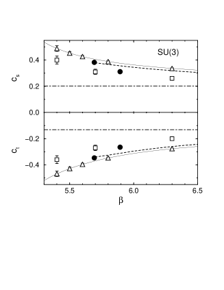
Figure 1: Anisotropy coefficients $c_{s}$ and $c_{t}$ for the $SU(2)$ and $SU(3)$ gauge theories.

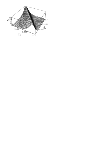
Figure 2: The Polyakov loop susceptibility for $SU(3)$ obtained on a $24^{3}\times 36\times 4$ lattice.

Table 1: Latent heat, pressure gap, $\Delta\langle P_{t}\rangle\left/\Delta\langle P_{s}\rangle\right.$ and $-r_{t}$ at the deconfining transition point of $SU(3)$ gauge theory.

lattice	$24^{2}\times 36\times 4$	$36^{2}\times 48\times 6$
$\beta$	5.6925	5.8936
$\Delta\epsilon/T^{4}$	2.074(34)	1.569(40)
$\Delta p/T^{4}$	0.001(15)	$-$0.003(17)
$\Delta\langle P_{t}\rangle\left/\Delta\langle P_{s}\rangle\right.$	1.201(35)	1.218(46)
$-r_{t}$	1.201(1)	1.220(3)

We first test the method for the case of $SU(2)$ gauge theory at the transition point $\beta_{c}$ for $N_{t}=4$ and 5. Simulations are performed on $16^{3}\times 4$ and $20^{3}\times 5$ lattices. Results for $c_{s}$ and $c_{t}$ are denoted by filled circles in Fig. 1 (top). Our results are consistent with the results from the integral method (doted curves) [5].

We then study the more realistic case of the $SU(3)$ gauge theory. Because the method works well even with data obtained only on isotropic lattices, we analyze the high statistics data by the QCDPAX Collaboration [11]. Simulations were performed at the deconfining transition point for $N_{t}=4$ and 6 on five lattices. Details of the $SU(3)$ simulations are given in [11].

Fig. 2 shows the $(\beta_{s},\beta_{t})$ dependence of the susceptibility on a $24^{2}\times 36\times 4$ lattice. Because the peak of the susceptibility becomes sharper as the spatial volume of the lattice is increased, we can measure $r_{t}$ most precisely on the spatially largest lattices. Therefore, in the following, we use the results obtained on the largest $24^{2}\times 36\times 4$ and $36^{2}\times 48\times 6$ lattices. The values obtained on smaller lattices are consistent. For the beta-function, we adopt a result computed from a recent string tension data [9].

In Fig. 1 (bottom), we summarize our results for the $c_{s}$ and $c_{t}$ of the $SU(3)$ gauge theory (filled circles) together with previous values: the perturbative results (dot-dashed lines) [1], results from the integral method (doted curves) [6], and those from the matching of Wilson loops on anisotropic lattices (squares [3], triangles [4]). We find that all non-perturbative methods give values which are roughly consistent with each other, showing a clear deviation from the perturbation theory.

The deconfining transition is of first order for $SU(3)$. At a first order transition point, we have a finite gap for energy density, the latent heat, but expect no gap for pressure. It is known that the perturbative anisotropy coefficients leads to a non-vanishing pressure gap at the deconfining transition point: $\Delta p/T^{4}=-0.32(3)$ and $-0.14(2)$ at $N_{t}=4$ and 6 [11].

New values for the gaps in $\epsilon$ and $p$ using our non-perturbative anisotropy coefficients are summarized in Table 1. We find that the problem of non-zero pressure gap is completely resolved with our non-perturbative anisotropy coefficients.

We note that, because the beta-function appears only as a common overall factor in (3) and (4), the conclusion that $\Delta p$ vanishes with our anisotropy coefficients does not depend on the value of the beta-function. Actually we have from eqs.(3) and (4) a simple condition for $\Delta p=0$:

$$\Delta\langle P_{t}\rangle\left/\Delta\langle P_{s}\rangle\right.=-r_{t}$$ (5)

where $\Delta\langle P_{s(t)}\rangle$ is the gap in the spatial (temporal) plaquette between the two phases. Although the two sides of (5) are obtained from quite different measurements, they agree precisely with each other as shown in Table 1.

We are grateful to J. Engels, T.R. Klassen and the members of CCP, Tsukuba for useful discussions. This work is in part supported by the Grants-in-Aid of Ministry of Education, Science and Culture (Nos. 08NP0101, 09304029, 10640248). SE is supported by JSPS.

References

- [1] F. Karsch, Nucl. Phys. B205 (1982) 285.
- [2] G. Burgers et al., Nucl. Phys. B304 (1988) 587.
- [3] J. Engels et al., Nucl. Phys. B (Proc. Suppl.) 63 (1998) 427.
- [4] T.R. Klassen, hep-lat/9803010.
- [5] J. Engels et al.,Nucl. Phys. B435 (1995) 295.
- [6] G. Boyd et al., Nucl. Phys. B469 (1996) 419.
- [7] S. Ejiri, Y. Iwasaki and K. Kanaya, hep-lat/9806007, to appear in Phys. Rev. D.
- [8] K. Akemi et al., Phys. Rev. Lett. 71 (1993) 3063.
- [9] R.G. Edwards et al., Nucl. Phys. B517 (1998) 377.
- [10] A.M. Ferrenberg and R.H. Swendsen, Phys. Rev. Lett. 61 (1988) 2635; 63 (1989) 1195.
- [11] Y. Iwasaki et al., Phys. Rev. D46 (1992) 4657.