THE INFRARED BEHAVIOUR OF THE GLUON PROPAGATOR FROM LATTICE QCD

Abstract

The gluon propagator in Landau gauge is calculated in quenched QCD on a large ($32^{3}\times 64$) lattice at $\beta=6.0$. In order to assess finite volume and finite lattice spacing artefacts, we also calculate the propagator on a smaller volume for two different values of the lattice spacing. New structure seen in the infrared region survives conservative cuts to the lattice data, and serves to exclude a number of models that have appeared in the literature.

1 Introduction

The infrared behaviour of the gluon propagator is important for an understanding of confinement. Several studies using Dyson–Schwinger equations [1, 2] have suggested that the gluon propagator diverges faster than $1/q^{2}$ in the infrared, and it has been claimed that this is a necessary condition for confinement. On the other hand, recent studies of coupled ghost and gluon Dyson–Schwinger equations [3, 4] indicate the gluon propagator vanishes in the infrared, in agreement with older studies [5, 6] using other methods. Other investigations [7] have also suggested a massive gluon, yielding an infrared finite propagator.

Lattice QCD should in principle be able to resolve this issue by first-principles, model-independent calculations. However, lattice studies have up to now been inconclusive,[8, 9] since they have not been able to access sufficiently low momenta. The lower limit of the available momenta on the lattice is given by $q_{\rm min}=2\pi/L$, where $L$ is the length of the lattice.

Here we will report results using a lattice with a length of 3.3 fm in the spatial directions and 6.7 fm in the time direction. This gives us access to momenta as small as 400 MeV.

2 Lattice formalism

The gluon field $A_{\mu}$ can be extracted from the link variables $U_{\mu}(x)$ using

$$U_{\mu}(x)=e^{ig_{0}aA_{\mu}(x+\hat{\mu}/2)}+{\cal O}(a^{3})\,.$$ (1)

Inverting and Fourier transforming this, we obtain

$$A_{\mu}(\hat{q}) \equiv \sum_{x}e^{-i\hat{q}\cdot(x+\hat{\mu}/2)}A_{\mu}(x+\hat{\mu}/2)$$ (2)

$$= \frac{e^{-i\hat{q}_{\mu}a/2}}{2ig_{0}a}\left[\left(U_{\mu}(\hat{q})-U^{\dagger}_{\mu}(-\hat{q})\right)-\frac{1}{3}{\rm Tr}\,\left(U_{\mu}(\hat{q})-U^{\dagger}_{\mu}(-\hat{q})\right)\right],$$

where $U_{\mu}(\hat{q})\equiv\sum_{x}e^{-i\hat{q}x}U_{\mu}(x)$ and $A_{\mu}(\hat{q})\equiv t^{a}A_{\mu}^{a}(\hat{q})$. The available momentum values $\hat{q}$ are given by

$$\hat{q}_{\mu}=2\pi n_{\mu}/(aL_{\mu}),\qquad n_{\mu}=0,\ldots,L_{\mu}-1$$ (3)

where $L_{\mu}$ is the length of the box in the $\mu$ direction. The gluon propagator $D^{ab}_{\mu\nu}(\hat{q})$ is defined as

$$D^{ab}_{\mu\nu}(\hat{q})=\langle A^{a}_{\mu}(\hat{q})A^{b}_{\nu}(-\hat{q})\rangle\,/\,V\,.$$ (4)

In the Landau gauge, the propagator is expected to have the form

$$D_{\mu\nu}^{ab}(\hat{q})=\delta^{ab}(\delta_{\mu\nu}-\frac{q_{\mu}q_{\nu}}{q^{2}})D(q^{2})\,,$$ (5)

where the new momentum variable $q$ is defined by

$$q_{\mu}\equiv\frac{2}{a}\sin\frac{\hat{q}_{\mu}a}{2},$$ (6)

such that at tree level, $D(q^{2})$ will have the simple form

$$D(q^{2})=1/q^{2}\,.$$ (7)

3 Simulation Parameters, Finite Size Effects and Anisotropies

We have analysed 75 configurations at $\beta=6.0$, on a $32^{3}\times 64$ lattice. Using the value of $a^{-1}=1.885$ GeV,[10] this corresponds to a physical volume of ($3.35^{3}\times 6.70$) fm. For comparison, we have also studied an ensemble of 125 configurations on a smaller volume of $16^{3}\times 48$, with the same lattice spacing. An accuracy of $\frac{1}{VN_{C}}\sum_{\mu,x}|\partial_{\mu}A_{\mu}|^{2}<10^{-12}$ was achieved for the Landau gauge condition on both lattices.

In the following, we are particularly interested in the deviation of the gluon propagator from the tree level form (7). We will therefore factor out the tree level behaviour and plot $q^{2}D(q^{2})$ rather than $D(q^{2})$ itself. Furthermore, in order to eliminate the most obvious source of lattice anisotropies, we will plot the data as a function of the momentum variable $q$ defined in (6).

     

Figure 1: Componentwise data, for the small lattice (left) and the large lattice (right). The filled triangles denote momenta directed along the time axis, while the filled squares denote momenta directed along one of the spatial axes.

Fig. 1 shows the gluon propagator as a function of $qa$ for both lattices, with momenta in different directions plotted separately. Only an averaging over the three spatial directions has been performed. For low momenta, there are large anisotropies in the small lattice data, due to finite size effects. This can be seen in particular from the difference between points representing momenta along the time axis and those representing momenta along the spatial axes for $qa\sim 0.4$ and $qa\sim 0.75$. These anisotropies are absent from the data from the large lattice, indicating that finite size effects here are under control.

However, at higher momenta, there are anisotropies which remain for the large lattice data, and which are of approximately the same magnitude for the two lattices. These anisotropies must be the result of finite lattice spacing errors in the action, which break down the continuum O(4) symmetry to the hypercubic symmetry. In order to eliminate these anisotropies, we select momenta lying within a cylinder of radius $\Delta\hat{q}a=2\times 2\pi/32$ along the 4-dimensional diagonals. The data surviving this cut are shown in fig. 2.

Figure 2: The gluon propagator from the large lattice. Only momentum vectors with a distance from the diagonals of 2 units of momenta or less have been kept. The solid circles denote those points which also lie within a cone with an opening angle of $20^{\circ}$.

We also consider a further cut, keeping only those momenta which lie within a cone of $20^{\circ}$ opening angle, directed along the diagonals and with its apex at the origin. This cut was found necessary to remove the low-momentum anisotropies on the small lattice.[11] The data surviving this cut are shown as filled symbols in fig. 2. It is interesting to see that even with this conservative cut, the main qualitative features of the data can still be observed.

4 Model Fits

We have considered the following functional forms:

$$D(q^{2}) = \frac{Z}{(q^{2})^{1+\alpha}+M^{2}}$$ (8)

$$D(q^{2}) = Z\left[(q^{2}+M^{2}(q^{2}))\ln\frac{q^{2}+4M^{2}(q^{2})}{\Lambda^{2}}\right]^{-1}$$ (9)

where $$M(q^{2})=M\left\{\ln\frac{q^{2}+4M^{2}}{\Lambda^{2}}/\ln\frac{4M^{2}}{\Lambda^{2}}\right\}^{-6/11}$$

$$D(q^{2}) = Z\left(\frac{A}{(q^{2}+M^{2})^{1+\alpha}}+\frac{1}{q^{2}+M^{2}}\right)$$ (10)

$$D(q^{2}) = Z\left(\frac{A}{(q^{2})^{1+\alpha}+(M^{2})^{1+\alpha}}+\frac{1}{q^{2}+M^{2}}\right)$$ (11)

$$D(q^{2}) = Z\left(Ae^{-(q^{2}/M^{2})^{\alpha}}+\frac{1}{q^{2}+M^{2}}\right)$$ (12)

Model (8) is the one used by Marenzoni et al. [9] Model (9) was proposed by Cornwall. [7] Models (10) and (11) are constructed as generalisations of (8) with the correct dimension and tree level behaviour in the ultraviolet regime.

All models were fitted to the large lattice data using the cylindrical cut. The lowest momentum value was excluded, as the volume dependence of this point could not be determined. In order to balance the sensitivity of the fit between the high- and low-momentum region, nearby data points within $\Delta(qa)<0.05$ were averaged.

Model (11) accounts for the data better than any of the other models. Fig. 3 shows $\chi^{2}$ per degree of freedom for fits to this model, as a function of the starting point of the fit (where the points are numbered 1, 2, …starting from the most infrared) and the number of points included in the fit. The region of interest is the right-hand section of the plots, where the number of points in the fit is large and the infrared region is included. (11) gives a good fit (with $\chi^{2}/{\rm dof}\sim 1$) for a wide range of momenta. Only when we try to include the most infrared points does $\chi^{2}/$dof go up to around 4.

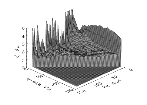
Figure 3: $\chi^{2}$ per degree of freedom for fits to model (11). The fits are to the large lattice data with the cylindrical cut, with nearby points averaged. The data points are numbered 1, …, 142, with the most infrared point being number 1. ‘Fit Width’ denotes the number of points included in the fit.

The parameter values for fits to (11) are shown in fig. 4. As long as a reasonable number of points, including points in the infrared region, are included in the fit, the values vary very little when the fitting interval is varied. Our best estimate for the parameters is

$$Z=1.21\raisebox{-1.72218pt}{$\stackrel{{\scriptstyle\scriptstyle+7}}{{\scriptstyle-4}}$}A=1.06\raisebox{-1.72218pt}{$\stackrel{{\scriptstyle\scriptstyle+1}}{{\scriptstyle-15}}$}\alpha=0.78\raisebox{-1.72218pt}{$\stackrel{{\scriptstyle\scriptstyle+9}}{{\scriptstyle-3}}$}M=0.38\raisebox{-1.72218pt}{$\stackrel{{\scriptstyle\scriptstyle+5}}{{\scriptstyle-2}}$}$$ (13)

where the errors denote the uncertainties in the last digit(s) of the parameters, due to fluctuations in the parameters as the fitting interval is varied.

Fig. 5 shows the fit to (11) using these parameters, as well as the best fits to the other models considered.

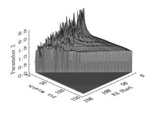
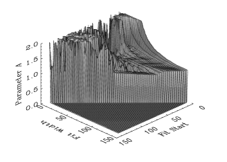
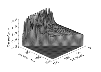
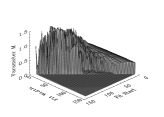
Figure 4: Parameter values for fits to model (11). The axes are as in fig. 3.

     

Figure 5: Fits to (a) model (11); (b) models (8) (dash–dotted line), (9) (dotted line), (10) (solid line) and (12) (dashed line).

5 Discussion and Outlook

We have evaluated the gluon propagator on an asymmetric lattice with a large physical volume. By studying the anisotropies in the data, and comparing the data with those from a smaller lattice, we have been able to conclude that finite size effects are under control on this lattice.

A clear turnover in the behaviour of $q^{2}D(q^{2})$ has been observed at $q\sim 1$GeV, indicating that the gluon propagator diverges less rapidly than $1/q^{2}$ in the infrared, and may be infrared finite or vanishing.

A more detailed study, including an investigation of the tensor structure and a detailed analysis of different functional forms, is in progress.[12] The effect of Gribov copies is also an important issue for consideration. In the future, we hope to use improved actions to perform realistic simulations at larger lattice spacings. This would enable us to evaluate the gluon propagator on larger physical volumes, giving access to lower momentum values.

References

- [1] S. Mandelstam, Phys. Rev. D 20, 3223 (1979)
- [2] N. Brown and M.R. Pennington, Phys. Rev. D 39, 2723 (1989)
- [3] L. von Smekal, A. Hauck, R. Alkofer, Phys. Rev. Lett. 79, 3591 (1997), hep-ph/9707327 (to appear in Ann. Phys.), and these proceedings.
- [4] D. Atkinson and J.C.R. Bloch, hep-ph/9712459; hep-ph/9802239 and these proceedings.
- [5] V.N. Gribov, Nucl. Phys. B 139, 19 (1978); D. Zwanziger, Nucl. Phys. B 378, 525 (1992)
- [6] M. Stingl, Phys. Rev. D 34, 3863 (1986); Phys. Rev. D 36, 651 (1987)
- [7] J. Cornwall, Phys. Rev. D 26, 1453 (1982)
- [8] C. Bernard, C. Parrinello, A. Soni, Phys. Rev. D49, 1585 (1994)
- [9] P. Marenzoni, G. Martinelli, N. Stella, Nucl. Phys. B 455, 339 (1995); P. Marenzoni et al, Phys. Lett. B 318, 511 (1993)
- [10] G.S. Bali and K. Schilling, Phys. Rev. D 47, 661 (1993)
- [11] D.B. Leinweber, C. Parrinello, J.I. Skullerud, A.G. Williams, hep-lat/9804015 (to be published in Phys. Rev. D)
- [12] D.B. Leinweber, C. Parrinello, J.I. Skullerud, A.G. Williams, in preparation.