CERN-TH/98-251
Moments of parton evolution probabilities on the lattice within the Schrödinger functional scheme

We define, within the Schrödinger functional scheme (SF), the matrix elements of the twist-2 operators corresponding to the first two moments of non-singlet parton densities. We perform a lattice one-loop calculation that fixes the relation between the SF scheme and other common schemes and shows the main source of lattice artefacts. This calculation sets the basis for a numerical evaluation of the non-perturbative running of parton densities.

CERN-TH/98-251

July 1998

1 Introduction

The evolution with the energy scale of hadronic structure functions can be computed within renormalization group improved perturbative QCD, but the calculation of their absolute normalization needs non-perturbative techniques. The lattice approach is a theoretically well established framework for non-perturbative estimates and various calculations of the first moments of hadronic structure functions have appeared in the literature [1]. The results show a discrepancy with experimental data already for the non-singlet structure functions [2, 3]. There are various sources of errors that may explain the disagreement. On the lattice side, possible systematic errors are the quenched approximation and the still rather large values of the bare coupling constant used in present simulations, or equivalently the rather low values of the lattice momentum cutoff, which prevent a correct estimate of the continuum limit. On the experimental side, structure functions are reliably parametrized by leading-twist operators only at large momentum transfers; a comparison at energy scales of a few GeV is affected by systematic errors due to higher-twist effects. A standard procedure is then to evolve the lattice results from the cutoff scale, a couple of GeV, to higher scales, where the comparison is safe. The evolution is done by using perturbative results for the renormalization constants of leading-twist operators on the lattice, which may be affected by the truncations of the perturbative series.

Non-perturbative estimates of renormalization constants have already been performed for local lowest-dimensional currents [4] and have been seen to be essential for a proper definition of the quark mass through chiral Ward identities or for disentangling the operator mixing entering the evaluation of hadronic matrix elements of the effective four-fermion weak Hamiltonians [5]. A possible method for evaluating these renormalization constants is based on the Schrödinger functional (SF): this method has been successfully applied to the study of non-perturbative running of the coupling constant and of the quark mass [6]. We intend to perform a similar non perturbative estimate of the running of leading-twist operators of hadronic structure functions in the SF scheme. Non-perturbative estimates of the running of parton densities are needed if the scale at which the hadron matrix element is renormalized is held fixed while the continuum limit is taken. In this case the ratio of the renormalization scale over the lattice cutoff becomes large, and a perturbative expansion of the leading logarithms of such a ratio is a priori not reliable.

The present paper defines the SF matrix elements of the first and second moments of non-singlet leading-twist operators and reports the results on the one-loop perturbative calculation. The calculation is useful to learn about the size of lattice artefacts and to fix those finite constants peculiar to the SF scheme that can be used to make contact with more common schemes such as minimal subtraction. In the first section we recall the basic features of the Schrödinger functional involving fermions, in the second we discuss the choice of the matrix element for twist-2 non-singlet operators, and in the third we report the results of our calculations and some concluding remarks.

2 The Schrödinger functional for fermions

This section is only meant to recall some basic facts that have been discussed exhaustively in the literature [7]. The Schrödinger functional represents the amplitude for the time evolution that takes into account quantum fluctuations of a classical field configuration between two predetermined classical states. It takes the form of a standard functional integral with fixed boundary conditions. It has been shown that its renormalizability properties are the same as those of the theory in an infinite volume, modulo the possible presence of a finite number of boundary counterterms. In QCD with fermions, it can be written as:

$$\mathcal{Z}[C^{{}^{\prime}},\bar{\rho}^{\prime},\rho^{\prime};C,\bar{\rho},\rho]=\int\mathcal{D}[U]\mathcal{D}[\psi]\mathcal{D}[\bar{\psi}]\rm{e}^{-S[U,\bar{\psi},\psi]}$$ (1)

where $C^{{}^{\prime}},C$ and $\bar{\rho}^{\prime},\rho^{\prime},\bar{\rho},\rho$ are the boundary values of the gauge and fermion fields respectively. In the following discussion the classical boundary gauge field will be set to zero. According to ref. [8] expectations values may involve the response to a variation of the classical Fermi field configurations on the boundaries $\zeta$:

$$\zeta({\bf{x}})=\frac{\delta}{\delta\bar{\rho}({\bf{x}})},\qquad\bar{\zeta}({\bf{x}})=-\frac{\delta}{\delta\rho({\bf{x}})}$$ (2)

$$\zeta^{\prime}({\bf{x}})=\frac{\delta}{\delta\bar{\rho}^{\prime}({\bf{x}})},\qquad\bar{\zeta}^{\prime}({\bf{x}})=-\frac{\delta}{\delta\rho^{\prime}({\bf{x}})}$$ (3)

as well as the fluctuating Fermi fields between the boundaries $\psi$. In the following we will use the same notations as in ref. [9]. By working out the functional integration in the presence of external sources one obtains the expression for the generating functional for all possible expectation values involving fermions, and in particular the basic non-zero contractions:

$$[\psi(x)\bar{\psi}(y)]_{F}=S(x,y)$$ (4)

$$[\psi(x)\bar{\zeta}({\bf{y}})]_{F}=S(x,y)U_{0}(y-a\hat{0})^{-1}P_{+}|_{y_{0}=a}$$ (5)

$$[\psi(x)\bar{\zeta}^{\prime}({\bf{y}})]_{F}=S(x,y)U_{0}(y)P_{-}|_{y_{0}=T-a}$$ (6)

$$[\zeta({\bf{x}})\bar{\psi}(y)]_{F}=P_{-}U_{0}(x-a\hat{0})S(x,y)|_{x_{0}=a}$$ (7)

$$[\zeta^{\prime}({\bf{x}})\bar{\psi}(y)]_{F}=P_{+}U_{0}(x)^{-1}S(x,y)|_{x_{0}=T-a}$$ (8)

 

$${[\zeta({\bf{x}})\bar{\zeta}({\bf{y}})]_{F}}$$

  (9)

$$[\zeta({\bf{x}})\bar{\zeta}^{\prime}({\bf{y}})]_{F}=P_{-}U_{0}(x-a\hat{0})S(x,y)U_{0}(y)P_{-}|_{x_{0}=a,y_{0}=T-a}$$ (10)

$$[\zeta^{\prime}({\bf{x}})\bar{\zeta}({\bf{y}})]_{F}=P_{+}U_{0}(x)^{-1}S(x,y)U_{0}(y-a\hat{0})^{-1}P_{+}|_{x_{0}=T-a,y_{0}=a}$$ (11)

 

$${[\zeta^{\prime}({\bf{x}})\bar{\zeta}^{\prime}({\bf{y}})]_{F}}$$

  (12)

where $P_{\pm}=\frac{1}{2}(1\pm\gamma_{0})$ and $S(x,y)$ is the fermion propagator satisfying:

$$(D+m_{0})S(x,y)=a^{-4}\delta_{xy},\qquad 0<x_{0}<T.$$ (13)

The operator $D$ is the lattice version of the covariant derivative. In this paper we will use the Wilson formulation where $D$ takes the form:

$$D=\frac{1}{2}\{\gamma_{\mu}(\bigtriangledown^{\dagger}_{\mu}+\bigtriangledown_{\mu})-a\bigtriangledown^{\dagger}_{\mu}\bigtriangledown_{\mu}\}$$ (14)

To one-loop approximation, the above expression must be expanded in perturbation theory up to order $g^{2}$ by expanding the gluon unitary matrix $U$ in terms of vector potentials $q$:

$$U_{\mu}(x)=\{1+gaq_{\mu}(x)+O(g^{2})\}$$ (15)

3 The correlations for non-singlet twist-2 operators

In the continuum, moments of non singlet structure functions are related, through the operator product expansion, to hadronic matrix elements of local twist-2 operators of the form:

$${\cal{O}}_{\mu_{1}\ldots\mu_{n}}^{qNS}=\bigl{(}\frac{i}{2}\bigl{)}^{n-1}{\bar{\psi}}(x)\gamma_{[\mu_{1}}\stackrel{{\scriptstyle\leftrightarrow}}{{D}}_{\mu_{2}}\cdots\stackrel{{\scriptstyle\leftrightarrow}}{{D}}_{\mu_{n}]}\frac{\lambda^{f}}{2}\psi(x)\ +\ \mbox{trace terms}$$ (16)

where $\stackrel{{\scriptstyle\leftrightarrow}}{{D}}_{\mu}$ is the covariant derivative, [“indices”] means symmetrization, and $p$ is the hadron momentum that can be assumed light-like up to power corrections of order $M^{2}/Q^{2}$ with $Q$ the four-momentum transfer of the vector boson probing the hadron structure.

The twist is defined from the difference between the engineering dimensions of the operator and its angular momentum. Indeed, all listed operators belong to irreducible representations of the angular momentum.

On the lattice, the discretization of the covariant derivative can be done in a standard way:

 

$${\bigtriangledown_{\mu}\psi(x)}$$

  (17)

but in general, owing to the lower (hypercubic) symmetry of the Euclidean lattice action with respect to that of the continuum ( all 4-d rotations), the identification of a given irreducible representation may require some particular combinations of operators. This classification has been discussed for example in refs. [10] and [11]. With the Schrödinger functional the symmetry is in general further reduced, from hypercubic to cubic, because of the fixed boundary conditions in time that mark this direction with respect to the others. In this paper, we will concentrate on the calculation of the first two moments to which we associate the following irreducible operators:

 

$${O^{q}_{12}}$$

  (18)

where $\lambda^{f}$ is a flavour matrix. These are a subset of the basis described in ref. [11], involving only spatial indices and are multiplicatively renormalizable. We define the matrix elements of the first two moments by the observables:

 

$${f_{0_{12}}(x_{0})}$$

  (19)

where the contraction of the classical fields is non-vanishing if the matrix $\Gamma$ satisfies: $\Gamma P_{-(+)}=P_{+(-)}$ and $p$ is the momentum of the classical field sitting on the boundary. They can be seen as the operator matrix elements between the vacuum and “$\rho$”-like classical state sitting at the $T=0$ boundary.

We take the limit of massless quarks, which in the numerical simulations can be monitored via axial Ward identities. In the SF framework it is possible to work at zero physical quark mass because a natural infrared cutoff to the Dirac operator eigenmodes is provided by the time extent of the lattice. This choice simplifies the recursive procedure at finite volume that leads to the reconstruction of the continuum non-perturbative renormalization constant of the operators.

The matrix element of the operator for the first moment involves two directions and three for the second moment. These directions must be provided by external vectors: we have chosen to obtain one of them from the contraction matrix $\Gamma$, i.e. from the polarization of the vector classical state:

$$\Gamma=\gamma_{k},\qquad k=1,2,3$$ (20)

and the remaining ones from the momentum $p$ of the classical Fermi field at the boundary. This choice gives for the tree level a non-vanishing matrix element in the massless quark limit, where we evaluate our correlations. The tree-level correlation can be easily calculated and reads, for the first moment:

$$f^{(0)}_{2}(x_{0})=\frac{i\mathaccent 23{p}_{1}N}{R(p)^{2}}\left[(-i\mathaccent 23{p}_{0})\left(M_{-}(p){\rm{e}}^{-2\omega({\bf{p}})x_{0}}-M_{+}(p){\rm{e}}^{-2\omega({\bf{p}})(2T-x_{0})}\right)\right]$$ (21)

where

$$\hat{p}_{\mu}=(2/a)\sin(ap_{\mu}/2),\qquad\mathaccent 23{p}_{\mu}=(1/a)\sin(ap_{\mu})$$ (22)

$$M(p)=m+\frac{1}{2}a\hat{p}^{2},\qquad M_{\pm}=M(p)\pm i\mathaccent 23{p}_{0}$$ (23)

$$\textrm{sinh }\left[\frac{a}{2}\omega({\bf{q}})\right]=\frac{a}{2}\left\{\frac{{\bf{\mathaccent 23{q}}}^{2}+(m+\frac{1}{2}a\hat{{\bf{q}}}^{2})^{2}}{1+a(m+\frac{1}{2}a\hat{{\bf{q}}}^{2})}\right\}^{\frac{1}{2}}$$ (24)

$$R(p)=M(p)\left\{1-\textrm{e}^{-2\omega({\bf{p}})T}\right\}-i\mathaccent 23{p}_{0}\left\{1+\textrm{e}^{-2\omega({\bf{p}})T}\right\}.$$ (25)

We have chosen for convention $\Gamma=\gamma_{2}$ and $\mathbb{p}=(p1,0,0)$. In the continuum and in the massless limit this expression reduces to:

$$f^{(0)}_{2}(x_{0})=\frac{Np_{1}}{(1+{\rm{e}}^{-2p_{1}T})^{2}}\left[{\rm{e}}^{-2p_{1}x_{0}}+{\rm{e}}^{-2p_{1}(2T-x_{0})}\right].$$ (26)

Notice that the symmetric choice $\Gamma=\gamma_{2}p2+\gamma_{1}p1$ and $\mathbb{p}=(p1,p2,0)$ would lead to:

 

$${f^{(0)}_{2}(x_{0})}$$

  (27)

which in the massless continuum limit reduces to

$$f^{(0)}_{2}(x_{0})=\frac{p_{1}^{3}p_{2}N}{(1+{\rm{e}}^{-2|{\bf{p}}|T})^{2}}\left(4{\rm{e}}^{-2|{\bf{p}}|T}\right)+\frac{p_{1}p_{2}^{3}N}{(1+{\rm{e}}^{-2|{\bf{p}}|T})^{2}}\left(4{\rm{e}}^{-2|{\bf{p}}|T}\right)$$ (28)

In the massless continuum limit, only the contribution proportional to $\exp(-2\omega T)$ survives, while at finite lattice spacing and for $x_{0}$ smaller than T the dominant term is $\exp(-2\omega x_{0})$, i.e. in this case the signal is dominated by lattice artefacts. Another advantage of using the non symmetric contraction is the economy in the number of non-zero momentum components.

The quantization of momenta on a finite lattice is one of the major sources of lattice artefacts. Indeed, with ordinary periodic boundary conditions the momentum cannot be chosen, in each direction, smaller than a minimum value proportional to the inverse lattice size. The presence of more independent momentum components increases the absolute value of the total momentum and therefore of the lattice artefacts associated to its size. In this respect, we will see that a different choice of boundary conditions can provide a “finite-size” momentum not submitted to quantization.

For the second moment, we choose $\Gamma=\gamma_{3}$ and $\mathbb{p}=(p1,p2,0)$. The tree-level expression in this case is just proportional to the one for the first moment:

$$f^{(0)}_{3}(x_{0})=\frac{\mathaccent 23{p}_{1}\mathaccent 23{p}_{2}N}{R(p)^{2}}\left[(i\mathaccent 23{p}_{0})\left(M_{-}(p){\rm{e}}^{-2\omega({\bf{p}})x_{0}}-M_{+}(p){\rm{e}}^{-2\omega({\bf{p}})(2T-x_{0})}\right)\right]=i\mathaccent 23{p}_{2}f^{(0)}_{2}(x_{0})$$ (29)

The observable is taken as the ratio of the correlation at one loop normalized by its tree-level expression and must be expurgated from the renormalization constant of the classical boundary fields $\zeta$. Following ref. [12], this is achieved through the normalization by the quantity called $f_{1}$, also normalized by its tree-level expression.

Finally, some care should be taken so as to ensure the massless quark limit at order $g^{2}$. The breaking of chiral simmetry of the Wilson action entails a non-zero shift of the quark mass from the naive value at order $g^{2}$:

$$m_{c}^{(1)}=-\frac{2}{3}\int_{-\pi}^{\pi}\frac{d^{4}q}{2\pi^{4}}\left\{\frac{1}{\hat{q}^{2}}\left[3+\frac{\hat{q}^{2}(4-\frac{1}{4}\hat{q}^{2})-\mathaccent 23{q}^{2}}{\mathaccent 23{q}^{2}+\frac{1}{4}(\hat{q}^{2})^{2}}\right]\right\}.$$ (30)

Including the mass shift simply amounts to a further contribution coming from the derivative of the tree-level expression calculated at the zero naive quark mass value times the coefficient of the order $g^{2}$ mass shift.

4 The results of the calculation

The expression for the observable at one loop in the continuum can be parametrized as:

 

$${{}Z(pL,x_{0}/L,a/L)=1+g^{2}Z^{(1)}(a/L)}$$

  (31)

where the scaling variables $pL$ and $x_{0}/L$ are kept constant when the number of lattice points is sent to infinity. Indeed, beyond the free field case, this limit does not exist because of the ultraviolet divergence manifested through the logarithmic term that breaks the free-field theory scale invariance. In the following, the momentum will be set to its minimum value, i.e. $pL=2\pi$.

The operator needs renormalization to be finite in the continuum limit: for example one can fix the operator matrix element equal to its tree-level value at $\mu=1/L$. At one loop one gets:

 

$${O^{R}(\mu)}$$

  (32)

The coefficients $b_{0},c_{0}$ are the interesting ones in the continuum limit, but at finite lattice spacing, i.e. with a finite number of lattice points, the correlation also contains corrections that decrease with the inverse powers of the number of points $N$. Our results are for the ordinary Wilson action without any improvement, and lattice artefacts start at order $1/N$ for both coefficients.

General formulae for calculating the perturbative expansion within the SF can be found in refs. [12, 9], where the correlation in eqs. (5 to 8) is calculated as:

$$\hbox{}\,\vbox{\halign{\strut\hfil$\displaystyle{#}$&&$\displaystyle{{}#}$\hfil\cr[\crcr}}\,\psi(x)\bar{\zeta}({\bf{y}})]_{F}=\frac{\delta\psi_{\rm{cl}}(x)}{\delta\rho({\bf{y}})}\cr[\psi(x)\bar{\zeta}^{\prime}({\bf{y}})]_{F}=\frac{\delta\psi_{\rm{cl}}(x)}{\delta\rho^{\prime}({\bf{y}})}\cr[\zeta({\bf{x}})\bar{\psi}(y)]_{F}=\frac{\delta\bar{\psi}_{\rm{cl}}(y)}{\delta\bar{\rho}({\bf{x}})}\cr[\zeta^{\prime}({\bf{x}})\bar{\psi}(y)]_{F}=\frac{\delta\bar{\psi}_{\rm{cl}}(x)}{\delta\bar{\rho}^{\prime}({\bf{y}})}$$ (33)

and in turn

 

$${\psi_{\rm{cl}}(x)}$$

  (34)

We have done the calculation independently by using the notion of $\psi_{\rm{cl}}$ and the explicit expressions of ref. [9] or by using directly the correlations given by eqs. 5 to 8 and the perturbative expansion of the Dirac propagator. In the latter case we obtain also diagrams where the gluon field emerges from the time links connecting the Dirac propagator to the zero time slice. In both cases the calculation was done in a time-momentum representation. The algebraic manipulations leading to the finite sums performed numerically were done with the algebraic program “FORM”.

The final Fortran result was obtained with double-precision accuracy. We have run all even lattice sizes ranging from 8 to 36 in the case of the first moment and to 40 for the second moment. The latter choice was forced by the slower approach to the continuum for the second moment. The fit to the $N$ dependence of our results has been made by the expression

$$Z^{(1)}(N)=B_{0}+C_{0}\ln(N)+\sum_{k=1,2}\frac{B_{k}+C_{k}\ln(N)}{N^{k}}\quad,{\rm{with}}\quad N=L/a,$$ (35)

excluding higher-order terms. The stability of the fit was checked against a change in the value of the smallest volume included. After checking the agreement to the per cent level with the expected value of the coefficient of the logarithm $C_{0}$, we fix it to its theoretical value and determine the remaining parameters. As an example, we report in Table $1$ the results for the first moment and for the correlations at $x_{0}=L/2$ of the constant $B_{0}$.

Range	Parameters	Constant	$\chi^{2}$
$24$–$34$	$5$	$0.0971$	$10^{-2}$
$22$–$34$	$5$	$0.0968$	$10^{-3}$
$20$–$34$	$5$	$0.0964$	$10^{-5}$

Table 1: Values of the constant of the correlation function of the first moment with $x_{0}=L/2$.

The values are shown for different fitting intervals and, in the last column, we report the $\chi^{2}$ values with a reference error of $10^{-5}$ on the theoretical points . An alternative determination can be achieved by making suitable combinations of the data where some of the dominant $1/L$ and $1/L^{2}$ corrections are eliminated. This leads to the results of Table 2, where we indicate the type of fitting coefficients eliminated from the general eq. and the fitting interval used.

Our final results for the constants, for the first and second moment, are in Table 3.

Range	Eliminated parameters	Constant	$\chi^{2}$
$24$–$30$	$\ln(N)/N,1/N,1/N^{2}$	$0.0967$	$1.5$
$24$–$30$	$\ln(N)/N,1/N$	$0.0967$	$10^{-2}$

Table 2: Values of the constant of the correlation function of the first moment with $x_{0}=L/2$ after elimination of some subleading contributions.

Moment	Definition	Constant
First	$x_{0}=L/4$	$B_{0}=0.084(1)$
First	$x_{0}=L/2$	$B_{0}=0.0967(5)$
Second	$x_{0}=L/4$	$B_{0}=0.010(5)$
Second	$x_{0}=L/2$	$B_{0}=0.008(2)$

Table 3: Values of the constants of the correlation functions $f_{2}$ and $f_{3}$ with the operator insertion at $x_{0}=L/2$ and $x_{0}=L/4$.

The approach to the continuum values is very slow, as can be seen from figures 1 and 2 where we compare the ratio of perturbative finite lattice coefficients with their continuum values for the two moments and the two $x_{0}$ cases.

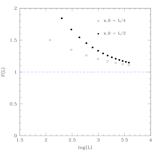
Figure 1: The ratio of perturbative finite lattice renormalization constant with their continuum value for the first moment in the two cases of $x_{0}=L/4(\circ)$ and $x_{0}=L/2(\bullet)$.

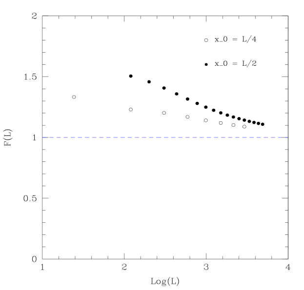
Figure 2: The ratio of perturbative finite lattice renormalization constants with their continuum value for the second moment in the two cases of $x_{0}=L/4(\circ)$ and $x_{0}=L/2(\bullet)$.

In the case of the second moment the slope of the approach is lower, indicating that momentum quantization is an important source of lattice artefacts. The continuum is approached from above in all cases, similarly to what happens for the proton matrix elements, by comparing the standard Wilson action with a partially non-perturbative $O(a)$ improvement [3].

The use of a physical momentum is not the only way to obtain non-vanishing matrix elements for the operators that we have considered. Indeed, the choice of periodic boundary conditions for fermions different from the usual ones [13]:

$$\psi(x)=\psi(x+L\hat{k})$$ (36)

to:

$$\tilde{\psi}(x)={\rm{e}}^{i\theta_{k}}\tilde{\psi}(x+L\hat{k})$$ (37)

where $\theta$ is an arbitrary constant phase, introduces a “finite-size momentum $\theta$” probed by the operator only when it involves fields on the two sides of the boundary that can play the same role as the ordinary momentum. One can also distribute the phase to all lattice points by an Abelian transformation on the Fermi fields:

$$\tilde{\psi}(x)={\rm{e}}^{i\frac{\theta}{L}x}\psi(x),$$ (38)

which changes the form of the lattice derivative from

 

$${\bigtriangledown_{\mu}\tilde{\psi}(x)}$$

  (39)

to:

 

$${\bigtriangledown_{\mu}\psi(x)}$$

  (40)

where

$$\lambda_{\mu}=e^{ia\theta_{\mu}/L},\qquad\theta_{0}=0,\qquad-\pi<\theta_{k}\leq\pi.$$ (41)

In this case the operator feels a “finite-size momentum $\theta/L$”at all lattice points. By taking the average of the operator insertion over all points, the same result is recovered.

We have repeated the perturbative calculation at zero momentum and non-zero “finite size momentum” $\theta=0.1/L$, to be compared with the minimal lattice momentum $p_{min}=2\pi/L$.

The lattice results converge much faster to their continuum limit, confirming the momentum quantization as a major source of lattice artefacts. Figures 3 and 4 show the ratio of lattice over continuum results also for this case.

Figure 3: The ratio of perturbative finite lattice renormalization constants with their continuum value for the first moment in the two cases of $x_{0}=L/4(\circ)$ and $x_{0}=L/2(\bullet)$ using “finite size momentum”.

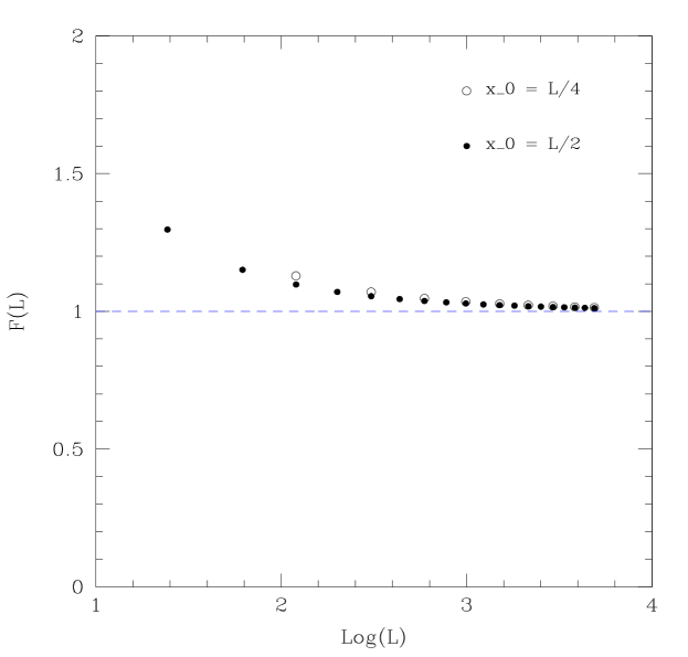
Figure 4: The ratio of perturbative finite lattice renormalization constants with their continuum value for the second moment in the two cases of $x_{0}=L/4(\circ)$ and $x_{0}=L/2(\bullet)$ using “finite size momentum”.

In this case also a global fit without elimination of subleading terms provides a very good estimate of the value of the constant. Our final best estimates are given in Table 4.

Moment	Definition	Constant
First	$x_{0}=L/4$	$B_{0}=-0.0577(1)$
First	$x_{0}=L/2$	$B_{0}=-0.4129(1)$
Second	$x_{0}=L/4$	$B_{0}=-0.2403(5)$
Second	$x_{0}=L/2$	$B_{0}=-0.747(2)$

Table 4: Values of the constants of the correlation functions $f_{2}$ and $f_{3}$ in the two definitions with the “finite size momentum”.

The result for the constant of the continuum limit of the quantity $f_{1}$ that subtracts the renormalization constants of the $\zeta$ fields from that of the operator is

$$B_{0}=-0.3590(1).$$ (42)

It has been obtained from fits to the data made available to us by P.Weisz.

Moment	Definition	Constant
First	$x_{0}=L/4(p\neq 0)$	$B_{0}=0.2635(10)$
First	$x_{0}=L/2(p\neq 0)$	$B_{0}=0.2762(5)$
Second	$x_{0}=L/4(p\neq 0)$	$B_{0}=0.1875(20)$
Second	$x_{0}=L/2(p\neq 0)$	$B_{0}=0.1895(50)$
First	$x_{0}=L/4(\theta\neq 0)$	$B_{0}=0.12180(15)$
First	$x_{0}=L/2(\theta\neq 0)$	$B_{0}=-0.23340(15)$
Second	$x_{0}=L/4(\theta\neq 0)$	$B_{0}=-0.06080(55)$
Second	$x_{0}=L/2(\theta\neq 0)$	$B_{0}=-0.5675(20)$

Table 5: Values of the constants of the operators renormalized in the two definitions with the real momentum $p$ or the “finite size momentum” $\theta$ different from zero.

Table 5 contains a summary of the constants $B_{0}$ for the operators, after removing the external legs renormalization, in the various cases that we have discussed.

We have shown by an explicit one-loop calculation the feasibility of a lattice evaluation of the renormalization constants of the first two non-singlet twist-2 operators within the Schrödinger functional scheme. The definition introduced in this paper is suitable for a finite-volume recursive scheme that can provide a full numerical reconstruction of the scale dependence of the renormalization constants, even in the non-perturbative regime. By comparing lattice and continuum perturbative estimates, we can conclude that lattice momentum quantization in a finite volume is one of the most important sources of lattice artefacts. The modification of fermion boundary conditions already introduced in the framework of the Symanzik improvement programme carried out by the ALPHA collaboration, introduces of a “finite-size momentum”, which escapes the quantization rule and turns out to substantially improve the approach to the continuum of our lattice results. Numerical studies with standard lattice momenta and with finite-size momenta are under way [14].

ACKNOWLEDGEMENTS.

We have considerably profited from the experience accumulated by the ALPHA collaboration with the Schrödinger functional with fermions. In particular, we thank K. Jansen, M. Lüscher, M. Testa and P. Weisz for many enlightening discussions and M. Lüscher for the access to some crucial internal notes of the ALPHA collaboration. We thank P. Weisz for providing us with the detailed perturbative results for “$f_{1}$”.

References

-
[1]
S. Capitani and G. Rossi,
Nucl. Phys. B433 (1995) 351
G. Martinelli et al., Nucl. Phys. B445 (1995) 81
M. Göckeler et al., Phys. Rev. D53 (1996) 2317
R. C. Brower et al., Nucl. Phys. B (Proc. Suppl.) 53 (1997) 547 -
[2]
L. Mankiewicz and T. Weigl,
Phys. Lett. B389 (1996) 334
-
[3]
C. Best et al.,
Hadron Structure Functions from Lattice QCD – 1997,
hep-ph/9706502 -
[4]
M. Lüscher, S. Sint, R. Sommer, H. Wittig,
Nucl. Phys. B491 (1997) 344
-
[5]
L. Conti et al.,
Nucl. Phys. B (Proc. Suppl.) 63 (1998) 880
-
[6]
M. Lüscher, R. Sommer, P. Weisz and U. Wolff,
Nucl. Phys. B389 (1993) 247; Nucl. Phys. B413 (1994) 481
S.Capitani et al., Nucl. Phys. B (Proc. Suppl.) 63 (1998) 153 -
[7]
M. Lüscher, R. Narayanan, P. Weisz and U. Wolff,
Nucl. Phys. B384 (1992) 168
S.Sint, Nucl. Phys. B421 (1994) 135 -
[8]
K. Jansen, C. Liu, M. Lüscher, H. Simma, S. Sint, R. Sommer,
P. Weisz and
U. Wolff, Phys. Lett. B372 (1996) 275
M. Lüscher, S. Sint, R. Sommer and P. Weisz, Nucl. Phys. B478 (1996) 365 - [9] M. Lüscher and P. Weisz, Nucl. Phys. B479 (1996) 429
-
[10]
M. Baake, B. Gemünden and R.Oedingen,
J. Math. Phys. 23 (1982) 944
J.E.Mandula, G.Zweig and J.Govaerts, Nucl. Phys. B228 (1983) 91 -
[11]
G. Beccarini, M. Bianchi, S. Capitani and G. Rossi,
Nucl. Phys. B456 (1995) 271
M.Göckeler et al., Phys. Rev. D54 (1996) 5705 - [12] S. Sint and P. Weisz, Nucl. Phys. B502 (1997) 251
- [13] M. Lüscher private communication,
- [14] K.Jansen, M.Guagnelli and R.Petronzio, work in progress