Topological properties of full QCD at the phase transition

Abstract

We investigate the topological properties of the QCD vacuum with 4 flavours of dynamical staggered fermions at finite temperature. To calculate the topological susceptibility we use the field–theoretical method. As in the quenched case, a sharp drop is observed for the topological susceptibility across the phase transition.

1 INTRODUCTION

The topological susceptibility is defined as

$$\chi\equiv\int d^{4}x\partial_{\mu}\partial_{\nu}\langle{\rm T}\left(K_{\mu}(x)K_{\nu}(0)\right)\rangle$$ (1)

where $K_{\mu}(x)$ is

$$K_{\mu}(x) = {g^{2}\over 16\pi^{2}}\epsilon_{\mu\nu\rho\sigma}\times$$ (2)

$$A_{\nu}^{a}\left(\partial_{\rho}A^{a}_{\sigma}-{1\over 3}gf^{abc}A_{\rho}^{b}A_{\sigma}^{c}\right)$$

and $Q(x)=\partial_{\mu}K_{\mu}(x)$ is the density of topological charge. Eq. (1) uniquely defines the prescription for the singularity of the time ordered product at $x\longrightarrow 0$ [1]. Determining $\chi$ around $T_{c}$ in full QCD is an important piece of information to test models of QCD vacuum [2].

1.1 The Simulation

We have simulated the theory on a $16^{3}\times 4$ lattice with four flavours of staggered fermions with bare mass $am=0.05$. We have used the HMC algorithm for the updating. To be sure that topology is well thermalized we have checked the topological charge of our sample of configurations by cooling. They are well decorrelated. In Fig. 1 we display the distribution of topological charge of our configurations at $\beta\equiv 6/g^{2}=5.04$. This histogram confirms that at this mass value the topology is well sampled [3]. We have learned that topology is easily decorrelated when we work with large quark masses [3, 4]. In our case also the lattice spacing is large, so that updating the instanton content is faster.

With our bare fermion mass and lattice size the deconfining transition is known to occur at $\beta_{c}=5.04$ [5]. We have checked this number by computing the Polyakov loop and the chiral condensate as shown in Fig. 2.

Figure 1: Distribution of topological charge $Q_{L}$ at $\beta=5.04$.

Figure 2: Polyakov loop (squares, right scale) and chiral condensate (circles, left scale) across the phase transition on a $16^{3}\times 4$ lattice.

The topological susceptibility was measured at $\beta$=5.00, 5.02, 5.04, 5.05, 5.06, 5.10.

Table 1: Topological susceptibility and $T/T_{c}$ vs. $\beta$.

	$\beta$	$T/T_{c}$	$\chi$/MeV4
	5.00	0.9677	1.61(43)
	5.02	0.9804	1.13(30)
	5.04	1.0000	1.21(30)
	5.05	1.0126	2.89(1.46)
	5.06	1.0274	1.63(1.22)
	5.10	1.1110	0.43(1.19)

1.2 The Operators

We have measured the topological susceptibility by using the 2–smeared lattice topological charge $Q_{L}$ [6]

$$Q_{L}(x)=-{1\over 2^{9}\pi^{2}}\sum\epsilon_{\mu\nu\rho\sigma}{\rm Tr}\left(\Pi_{\mu\nu}(x)\Pi_{\rho\sigma}(x)\right)$$ (3)

and the field–theoretical method [7] to extract $\chi$ from the lattice susceptibility

$$\chi_{L}\equiv{Q_{L}^{2}\over V}=Z^{2}a^{4}\chi+M$$ (4)

where $Q_{L}$ is the lattice total charge $Q_{L}\equiv\sum_{x}Q_{L}(x)$ and $V$ the space–time volume. The multiplicative and additive renormalizations $Z$ and $M$ have been evaluated by use of the heating method [8, 9].

2 DETERMINATION OF $a$, $Z$ AND $M$

The lattice spacing was extracted by measuring the string tension at $\beta=5.00$, 5.04 and 5.10 on a $16^{4}$ lattice. For the other values of $\beta$ it was determined by a splines interpolation. Wilson loops were evaluated by using smeared spatial links. From the value at $\beta_{c}$ ($a=0.300(20){\rm fm}$) we infer the critical temperature to be $T_{c}=164(11)$ MeV.

The heating method to evaluate $Z$ and $M$ yields a non–perturbative determination of these renormalization constants [8, 9]. To calculate $Z$ a local updating algorithm is applied on a configuration containing a charge +1 classical instanton. These updatings, being local, thermalize the short distance fluctuations, responsible for the renormalization effects, and due to the slowing down leave large structures, like instantons, unchanged. The measurement of $Q_{L}$ on such updated configurations yields $Z\cdot Q$. As $Q$ is known, one can extract $Z$. Notice that this procedure is equivalent to imposing the continuum value for the 1–instanton charge (in the $\overline{\rm MS}$ scheme it is +1) and extracting the finite multiplicative renormalization $Z$ by evaluating a matrix element of $Q_{L}$.

The additive renormalization $M$ is obtained in a similar way. We apply a few heating steps with a local updating algorithm on a zero–field configuration. Then the topological susceptibility is calculated. This provides the value of $M$, if no instantons have been created during the few updating steps. This method agrees with the treatment of the singularity of Eq.(1).

As explained in [9], cooling tests must be done to check that the background topological charge has not been changed during the local heating (it is +1 in the calculation of $Z$ and 0 in the evaluation of $M$).

3 RESULTS

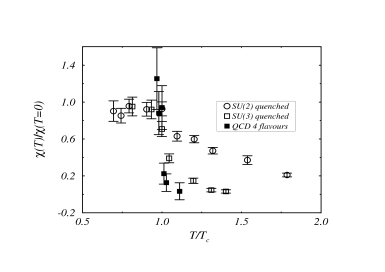
The values for the topological susceptibility and the temperature are given in table 1. In Fig. 3 we show the normalized topological susceptibility $\chi(T)/\chi(T=0)$ as a function of the temperature. The value at zero temperature $\chi(T=0)$ has been obtained by averaging the values at $T<T_{c}$. In the same figure the results for the quenched case [9, 10] are shown for comparison. The signal for $\chi$ drops strongly when crossing the transition temperature. Analogous results have been reported for two flavours and by using the cooling method [11].

From our data we cannot yet conclude that the drop in presence of fermions is steeper than for the quenched case, especially after considering that our simulations have been done at low beta values, where a poor scaling is expected, with a possible resulting large systematic effect on the scale $T/T_{c}$.

Comparing the full QCD results to the quen-ched case is an important issue for testing instanton liquid models of the vacuum. In view of that we are adding determinations on a $32^{3}\times 8$ lattice where we expect better control on scaling.

Figure 3: Behaviour of the topological susceptibility as a function of the normalized temperature $T/T_{c}$.

4 Acknowledgements

A. Di Giacomo acknowledges the financial contribution of the European Commission under the TMR-Program ERBFMRX-CT97-0122.

References

- [1] E.Witten, Nucl. Phys. B156 (1979) 269.
- [2] E. Shuryak and T. Schafer, Ann. Rev. Nucl. Part. Sci. 47 (1997) 359.
- [3] B. Allés, G. Boyd, M. D’Elia, A. Di Giacomo and E. Vicari, Phys. Lett. B389 (1996) 107.
- [4] B. Allés et al., hep-lat/9803008.
- [5] F. R. Brown et al., Phys. Lett. B251 (1990) 181.
- [6] C. Christou, A. Di Giacomo, H. Panagopoulos and E. Vicari, Phys. Rev. D53 (1996) 2619.
- [7] M. Campostrini, A. Di Giacomo, H. Pana-gopoulos and E. Vicari, Nucl. Phys. B329 (1990) 683.
- [8] A. Di Giacomo and E. Vicari, Phys. Lett. B275 (1992) 429.
- [9] B. Allés, M. D’Elia and A. Di Giacomo, Nucl. Phys. B494 (1997) 281.
- [10] B. Allés, M. D’Elia and A. Di Giacomo, Phys. Lett. B412 (1997) 119.
- [11] P. de Forcrand, M. García Pérez, J. E. Hetrick and I.-O. Stamatescu, Nucl. Phys. B (Proc. Suppl.) 63A-C (1998) 549.