Finite Size Analysis of the $U(1)$ Phase Transition using the World-sheet Formulation

Abstract

We present a high statistics analysis of the pure gauge compact U(1) lattice theory using the the $world-sheet$ or Lagrangian $loop$ representation. We have applied a simulation method that deals directly with (gauge invariant) integer variables on plaquettes. As a result we get a significant amelioration of the simulation that allows to work with large lattices avoiding the metaestability problems that appear using the standard Wilson formulation.

I Introduction

It is well known that pure $U(1)$ lattice gauge theory exhibits a phase transition separating a region where photons remain confined (strong coupling regime) and a Coulombian region (weak coupling). Nevertheless, the order of such transition is rather controversial [1, 2]. Simulations on hypercubical lattices using the Wilson form of the action shown the existence of a latent heat that seems to persist in the infinite volume limit [3, 4].If this transition is actually of first order, hence the gauge U(1) lattice theory would be lacking of a continuum limit.

The seriousness of such a situation has motivated the appearance of two lines of study. The first one is intended to check if the unexpected first order nature of this phase transition is an “accident” of the simulation, originated by the imposition of an hypercubical lattice [5], the periodic boundary conditions [6], etc. The second line of work goes directly to the the physical origin of the phase transition, the monopole condensation [7], and to the analysis of all related effects, as the presence of monopole percolation [8], that can shadow the behavior of the phase transition.

Although the formulation of the compact pure gauge U(1) theory on a lattice is very simple, i.e. there are only phases associated to the links, obtaining reliable numerical results from simulations is a rather difficult task. The earlier numerical simulations of such a theory indicated actually a continuous phase transition [9, 10]. The evidences which favor a first order transition appeared only when larger lattices and higher statistics were accessible [11, 12, 13].However, numerical simulations on larger lattices are very difficult. This is originated mainly by the lack of tunneling between phases that become incredibly stable and difficult the statistical analysis.

The ordinary Wilson formulation of QED has the links as the basic variables representing the gauge field and therefore involves a gauge redundancy. A different implementation of QED on the lattice which avoid the gauge redundancy can be attained using a description directly in terms of the world-sheets of gauge invariant quantities or loop excitations. This is the Lagrangian counterpart of the former introduced Hamiltonian loop representation [14, 15]. Although the non-canonical nature of the loop algebra had made elusive this Lagrangian formulation, in a previous set of papers [16, 17] a procedure to cast loops into the so-called world-sheet formulation was introduced.

In this paper we present a large statistics analysis of the pure gauge U(1) lattice theory using the world-sheet formulation. The lattice action used is equivalent to the Villain form. In this formulation basic variables are integer variables on the plaquettes. As we will comment, the thermodynamical behavior over the phase transition is different to the one obtained from a standard simulation. The persistent metaestability problems that appear in the simulations using the traditional formulation are absent in the case of the world-sheet formulation . This therefore makes this formulation a useful computational tool.

The plan of the paper is as follows. In Sec. II we summarize the basics of the world-sheet approach. In Sec. III we present the simulation method and the results using the world-sheet action corresponding to the Villain U(1) theory. Sec. IV is devoted to the analysis of the critical exponents of the transition. Finally, sec. V contains the summary of the work and the main conclusions.

II The Lagrangian Loop Approach or the World-Sheet Formulation

QCD is generally defined in terms of local fields, quarks and gluons, but the physical excitations are extended composites: mesons and baryons. There is an alternative quantum formulation of Yang-Mills theories directly in terms of these extended excitations namely, the loop representation [14, 15]. The basis of the loop description of gauge theories can be traced to the idea of describing gauge theories explicitly in terms of Wilson loops or holonomies [18, 19, 20] since Yang [21] noticed their important role for a complete description of gauge theories. Loops replace the information furnished by the vector potential. A description in terms of loops or strings, besides the general advantage of only involving the gauge invariant physical excitations, is appealing because all the gauge invariant operators have a simple geometrical meaning when realized in the loop space.

The loop based approach of ref. [14, 15] describes the quantum electrodynamics in terms of the gauge invariant holonomy (Wilson loop)

$$\hat{W}(\gamma)=\exp[ie\oint_{\gamma}A_{a}(y)dy^{a}],$$ (1)

and the conjugate electric field $\hat{E}^{a}(x)$ . They obey the commutation relations

$$[\hat{E}^{a}(x),\hat{W}(\gamma)]=e\int_{\gamma}\delta(x-y)dy^{a}\hat{W}(\gamma).$$ (2)

These operators act on a state space of Abelian loops $\psi(\gamma)$ that may be expressed in terms of the transform

$$\psi(\gamma)=\int d_{\mu}[A]<\gamma\mid A><A\mid\psi>=\int d_{\mu}[A]\psi[A]\exp[-ie\oint_{\gamma}A_{a}dy^{a}].$$ (3)

This loop representation has many appealing features: first, it allows to do away with the first class constraints of gauge theories. That is, the Gauss law is automatically satisfied. Second, the formalism only involves gauge invariant objects. Third, all the gauge invariant operators have a transparent geometrical meaning when they are realized in the loop space.

When this loop representation is implemented in the lattice it offers a gauge invariant description of physical states in terms of kets $\mid C>=\hat{W}(C)\mid 0>$, where $C$ labels a closed path in the spatial lattice. Eq.(2) becomes

$$[\hat{E}_{l},\hat{W}(C)]=N_{l}(C)\hat{W}(C),$$ (4)

where $l$ denotes the links of the lattice, $\hat{E}(l)$ the lattice electric field operator, $\hat{W}(C)=\prod_{l\in C}\hat{U}(l)$ and $N_{l}(C)$ is the number of times that the link $l$ appears in the closed path $C$.

In this loop representation, the Wilson loop acts as the loop creation operator:

$$\hat{W}(C^{\prime})\mid C>=\mid C^{\prime}\cdot C>.$$ (5)

The physical meaning of a loop may be deduced from (4) and (5), in fact

$$\hat{E}_{l}\mid C>=N_{l}(C)\mid C>,$$ (6)

which implies that $\mid C>$ is an eigenstate of the electric field. The corresponding eigenvalue is different from zero if the link $l$ belongs to $C$. Thus $C$ represents a line of electric flux.

In order to cast the loop representation in Lagrangian form it is convenient to use the language of differential forms on the lattice of ref. [22]. Besides the great simplifications to which this formalism leads its advantages consists in the general character of the expressions obtained. That is, most of the transformations are independent of the space-time dimension or of the rank of the fields. So let us summarize the main concepts and some useful results of the differential forms formalism on the lattice.

A k-form is a function defined on the k-cells of the lattice (k=0 sites, k=1 links, k=2 plaquettes, etc.) over an Abelian group which shall be R, Z, or U(1)=reals module 2$\pi$. Integer forms can be considered geometrical objects on the lattice. For instance, a 1-form represents a path and the integer value on a link is the number of times that the path traverses this link. $\nabla$ is the co-border operator which maps k-forms onto (k+1)-forms. It is the gradient operator when acting on scalar functions (0-forms) and it is the rotational on vector functions (1-forms). We shall consider the scalar product of p-forms defined $<\alpha\mid\beta>=\sum_{c_{k}}\alpha(c)\beta(c)$ where the sum runs over the k-cells of the lattice. Under this product the $\nabla$ operator is adjoint to the border operator $\partial$ which maps k-forms onto (k-1)-forms and which corresponds to minus times the usual divergence operator. That is,

$$<\alpha\mid\nabla\beta>=<\partial\alpha\mid\beta>,$$ (7)

$$<\nabla\alpha\mid\beta>=<\alpha\mid\partial\beta>.$$ (8)

The co-border $\nabla$ and border $\partial$ operators verify

$${\nabla}^{2}=0,\;\;{\partial}^{2}=0.$$ (9)

The Laplace-Beltrami operator operator is defined by

$$\Box=\nabla\partial+\partial\nabla.$$ (10)

It is a symmetric linear operator which commutes with $\nabla$ and $\partial$, and differs only by a minus sign from the current Laplacian $\Delta_{\mu}\Delta_{\mu}$. From Eq.(10) is easy to show the Hodge-identity:

$$1=\partial{\Box}^{-1}\nabla+\nabla{\Box}^{-1}\partial.$$ (11)

After this parenthesis on differential forms on the lattice let us consider the generating functional for the Wilson lattice U(1) action:

$$Z_{W}=\int_{-\pi}^{\pi}(d\theta_{l})\exp(-\frac{\beta}{2}\sum_{p}\cos{\theta}_{p}),$$ (12)

where the subscripts $l$ and $p$ stand for the lattice links and plaquettes respectively.

Fourier expanding the $\exp[\cos\theta]$ we get

$$Z_{W}=\int_{-\pi}^{\pi}(d\theta_{l})\prod_{p}\sum_{n_{p}}I_{n_{p}}(\beta)e^{in_{p}{\theta}_{p}},$$ (13)

which can be written, using the differential forms language as

$$Z_{W}=\sum_{\left\{n_{p}\right\}}\int_{-\pi}^{\pi}(d\theta_{l})\exp(\sum_{p}\ln I_{n_{p}}(\beta))e^{i<n,\nabla\theta_{l}>}.$$ (14)

In the above expression, $\theta_{l}$ is a real periodic 1-form, that is, a real number $\theta\in[-\pi,\pi]$ defined on each link of the lattice; $\nabla$ is the co-border operator; $n_{p}$ are integer 2-forms, defined at the lattice plaquettes. By eq. (8) and integrating over $\theta_{l}$ we obtain a $\delta(\partial n_{p})$. Then, the partition function can be written as

$$Z_{W}\propto\sum_{\left\{n_{p};\partial n_{p}=0\right\}}\exp(\sum_{p}\ln I_{n_{p}}(\beta)),$$ (15)

the constraint $\partial n_{p}=0$ means that the sum is restricted to $closed$ 2-forms. Thus, the sum runs over collections of plaquettes constituting closed surfaces.

An alternative and more easy to handle lattice action than the Wilson action is the Villain action. The partition function for this action is given by

$$Z_{V}=\int(d\theta)\sum_{s}\exp(-\frac{{\beta}_{V}}{2}\mid\mid\nabla\theta-2\pi s\mid\mid^{2}),$$ (16)

where $\mid\mid\ldots\mid\mid^{2}=<\ldots,\ldots>$. If we use the Poisson summation formula

$$\sum_{s}f(s)=\sum_{n}\int_{-\infty}^{\infty}d\phi f(\phi)e^{2\pi i\phi n}$$

and we integrate the continuum $\phi$ variables we get

$$Z_{V}=(2\pi{\beta}_{V})^{-N_{p}/2}\int(d\theta)\sum_{n}\exp(-\frac{1}{2{\beta}_{V}}<n,n>+i<n,\nabla\theta>),$$ (17)

where $N_{p}$ in the number of plaquettes of the lattice. Again, we can use the equality: $<n,\nabla\theta>=<\partial n,\theta>$ and integrating over $\theta$ we obtain a $\delta(\partial n)$. Hence we get:

$$Z_{V}=(2\pi{\beta}_{V})^{-N_{p}/2}\sum_{\left\{n;\partial n=0\right\}}\exp(-\frac{1}{2{\beta}_{V}}<n,n>),$$ (18)

where $n$ are integer 2-forms. Eq. (18) is obtained from Eq.(15) in the $\beta\rightarrow\infty$ limit.

If we consider the intersection of one of such surfaces with a $t=constant$ plane we get a loop $C_{t}$. It is easy to show that the creation operator for this loop is just the creation operator for the loop representation i.e. the Wilson loop operator. Repeating the steps from Eq.(16) to Eq.(18) we get for $<\hat{W}(C_{t})>$

$$<W(C_{t})>=\frac{1}{Z}(2\pi{\beta}_{V})^{-N_{p}/2}\sum_{\begin{array}[]{c}n\\ \left(\partial n=C_{t}\right)\end{array}}\exp(-\frac{1}{2{\beta}_{V}}<n,n>).$$ (19)

This is a sum over all world-sheets spanned on the loop $C_{t}$. In other words, we have arrived to an expression of the partition function of compact electrodynamics in terms of the world-sheets of pure electric loop excitations. Notice that the loop action corresponding to the Villain action is proportional to the $quadratic$ $area$ $A_{2}$:

$$S_{L}=-\frac{1}{2{\beta}_{V}}A_{2}=-\frac{1}{2{\beta}_{V}}\sum_{p\in{\cal S}}n_{p}^{2}=-\frac{1}{2{\beta}_{V}}<n,n>,$$ (20)

i.e. the sum of the squares of the multiplicities $s_{p}$ of plaquettes which constitute the loop’s world sheet ${\cal S}$. It is interesting to note the similarity of this action with the continuous Nambu action or its lattice version, the Weingarten action [23], which is proportional to the area swept out by the bosonic string.

III Numerical analysis

We simulated the loop lattice action of eq. (20). In ref. [16] we shown that this action is equivalent to the Integer Gaussian Model (IGM) that, in turn, it can be also reached as a limit of the non compact scalar QED in the limit of infinite Higgs coupling. In that paper we presented a direct simulation of the IGM which from the analysis of the energy histograms showed clearly the first order nature of the transition. Nevertheless, we did not computed the critical exponents of the phase transition.

Here we have performed a more quantitative study and computed the exponents of the phase transition. We applied the simulation method introduced in ref.[17]. This method consists in generating collections of integer variables attached to plaquettes which form surfaces with the appropriate constraints for each model (null frontier in the present pure gauge case). The variables are updated by means of a standard Metropolis Monte Carlo algorithm. These larger simulations produced a phase transition for the coupling constant $\beta=1/(2\beta_{V})=0.778$ i.e. $\beta_{V}=1/(2*0.778)=0.6426$ which is slightly higher than the previous value of $\beta_{V}\simeq 0.64$ [17].

The physical magnitudes measured under the simulation are the internal energy and the specific heat both normalized to the number of plaquettes $N_{p}=6L^{4}$:

$$e = N_{p}^{-1}\langle E\rangle$$ (21)

$$C_{v} = \beta^{2}N_{p}^{-1}\left(\langle E^{2}\rangle-\langle E\rangle^{2}\right)$$ (22)

on $\beta\equiv{1}/{2\beta_{V}}$.

The details of the run are the following:

• Hypercubical lattice (that is, periodic boundary conditions)

• Sizes ranging from $L=8$ to $L=24$.

• Good statistics, more than 100 times the self-correlations. It means millions of iterations for $L=24$.

• In order to locate the transition and the specific heat peaks, we didn’t do thermal cycles. Instead we used iteratively Ferrenberg-Swedsen reweighting until a two peaks histogram were found.

We made a FSS analysis for the following quantities:

• The specific heat maxima $C_{max}(L)$ (§IV A).

• The critical coupling position $\beta_{c}(L)$ (§IV B).

• The partition function zeroes in the complex plane. (§IV C).

• The latent heat, that is the distance between the two peaks (§IV D).

The calculations have been performed in Pentium computers running Linux (including the RTNN machine of 32 Pentium Pro processors at 200MHz). As it is expected, the elapsed time in the runs grows with the volume of the lattice obeying the following relation:

$$t=42\left(\frac{L}{10}\right)^{4}\mbox{hours/Mit},$$ (23)

where $t$ is the elapsed time for a Pentium Pro 200MHz running a million of iterations.

We have been very careful with the statistical analysis of such a transition. We have measured the autocorrelations, $\tau_{e}$, of the time-series for each lattice size in order to determine both, the number of thermalization iterations and the number of measures to obtain a significative number of independent measures. It is accepted [24] that about $20\tau_{e}$ iterations are enough in order to have the series thermalized and about $100\tau_{e}$ to have a sufficiently large time series. Table I collects this data.

$L$	$\beta_{MC}$	$\tau$	$n_{\rm{th}}/\tau$	$n_{\rm{m}}/\tau$
6	0.77991	90	1100	110000
8	0.77821	300	330	660
10	0.77821	500	100	200
12	0.77700	810	70	140
14	0.77700	1500	60	100
16	0.77688	2100	50	225
18	0.77688	3300	40	130
20	0.77688	5000	30	110
24	0.77680	13100	20	100

TABLE I.: Correlations

Using this data, one obtains that the self-correlation time grows exponentially (critical slowing down) according to

$$\tau=\tau_{0}e^{2\sigma L}\qquad\tau_{0}=49(4)\quad\sigma=0.116(2)\quad{\cal Q}=0.95,$$ (24)

where we supposed an error of about a 5% measuring $\tau$.

The goodness of the fits is done using

$${\cal Q}=Q\left(\frac{d.o.f}{2},\frac{\chi^{2}}{2}\right)$$ (25)

where $Q(a,x)$ is the regularized gamma function

$$Q(a,x)\equiv 1-P(a,x)\equiv\frac{\Gamma(a,x)}{\Gamma(a)}\equiv\frac{1}{\Gamma(a)}\int_{x}^{\infty}e^{-t}t^{a-1}dt.$$ (26)

Combining (23) and (24) we obtain the CPU times needed for an arbitrary simulation. We spent about three months of calculations for $L=24$, and a simple estimation reveals that to calculate $L=28$ in our machine we would need more than a year.

In Fig. 1 one can see energy histograms for different lattice sizes an the time series showing the presence of tunneling between the two phases. This undoubtedly shows that the world-sheet formulation (in terms of integer variables on plaquettes) is considerable more effective than the standard one (in terms of gauge potentials on links) to carry out a simulation.

FIG. 1.: Some Monte Carlo runs with their corresponding histograms for $L=12,16,20,24$. All the axes are equally scaled in order to compare them. Notice that for large $L$ the separation between phases grows, that is, the two peaks structure is more clear and in the time-series, the chance for tunneling decreases.

IV Critical exponents

Table II summarizes all the observables measured in this work.

$L$	$\beta_{MC}$	$\beta_{c}$	$\eta^{(0)}$	$10^{-3}\cdot\chi^{(0)}$	$C_{v}^{max}$		$\Delta e$
6	0.77991	0.7806(5)	0.780215(2)	9.9(2)	3.	4750(7)	-
8	0.77821	0.7785(4)	0.778358(3)	4.3(1.8)	5.	42(6)	-
10	0.77821	0.7780(2)	0.777978(4)	2.0(2)	8.	44(9)	0.0237(5)
12	0.77700	0.7770(2)	0.776985(1)	1.2(2)	10.	2(3)	0.0206(4)
14	0.77700	0.7769(7)	0.776972(8)	0.76(2)	14.	7(4)	0.019(1)
16	0.77699	0.7769(5)	-	-	20.	1(5)	0.0169(1)
18	0.77688	0.7768(2)	0.776843(2)	0.36(3)	24.	2(2)	0.0155(2)
20	0.77688	0.7768(8)	-	-	36.	2(7)	0.0160(5)
24	0.77680	0.7767(7)	-	0.23(2)	65.	8(1.8)	0.0145(4)

TABLE II.: Observables measured in this work. 1st an 2nd column contain the size of the lattice and $\beta_{MC}$ of the run. 3rd column contains the value of the coupling, $\beta_{c}$, of the maximum of $C_{v}$. In 4th and 5th columns one can find the real and imaginary part of the coupling that vanishes $Z$. 6th column contains $C_{v}$ and finally 7th column is the latent heat, $\Delta e$.

A Specific heat

In a 1st order phase transition, the specific heat is expected to have a volume scaling law, i.e.

$$C_{v}^{max}(L)=a_{1}+b_{1}L^{D}.$$ (27)

But a continuous phase transition must obey

$$C_{v}^{max}(L)=a_{2}+b_{2}L^{\alpha/\nu}.$$ (28)

Both expressions are equal if $\alpha=1$ and $\nu=1/D$. Using the data collected in column 6 of the table II we have performed a fit according to those scaling laws. Results are summarized in table III.

	1st order, eq. (27)					2nd order, eq. (28)
$L$	$a_{1}$		$10^{-4}b_{1}$	$\chi^{2}/_{d.o.f}$	${\cal Q}$	$\alpha/\nu$	$\chi^{2}/_{d.o.f}$	${\cal Q}$
6-24	3.	16(6)	$2.5(3)$	$2.9\cdot 10^{2}$	$0.51\cdot 10^{-375}$	2.44(4)	18.8	$0.97\cdot 10^{-18}$
8-24	5.	08(5)	$2.1(3)$	$7.3\cdot 10$	$0.38\cdot 10^{-76}$	2.7(7)	19.2	$0.91\cdot 10^{-15}$
10-24	6.	7(1)	$1.9(3)$	5.1	$0.43\cdot 10^{-3}$	3.60(13)	1.5	0.22
12-24	7.	7(3)	$1.8(3)$	2.8	$0.38\cdot 10^{-1}$	3.4(2)	1.6	0.19
14-24	8.	6(4)	$1.7(5)$	$5.8\cdot 10^{-2}$	0.94	3.9(3)	0.079	0.78
16-24	8.	8(9)	$1.7(6)$	$6.2\cdot 10^{-3}$	0.94	-	-	-

TABLE III.: Fits of $C_{v}^{max}$. The 1st order fit was done using eq. (27) (growing proportional to $L^{D}$). 2nd order fit corresponds to eq. (28), that is, growing as $L^{\alpha/\nu}$, being $\alpha/\nu$ free. Notice that in both cases the best fits are obtained using only the values $14<L<24$. In addition, the best 2nd order fit gives and exponent close to 4.

FIG. 2.: FSS of the specific heat as a function of the volume. The points with error bars are the data and the solid line is the fit of eq. (27) using the three last points. Notice that the smaller lattices are away from this fit.

Fig. 2 shows the measured values of $C_{v}^{max}$ as a function of $L^{4}$. Notice the alignment of the points, exhibiting a 1st order behavior. Solid line is the 1st order fit using only values $14<L<24$.

B Critical coupling

The critical coupling must reach their asymptotic behavior obeying the following laws,

$$\beta_{c}(L)=\beta_{c}(\infty)+AL^{-1/\nu}\quad\text{(2nd order),}\quad\beta_{c}(L)=\beta_{c}(\infty)+AL^{-D}\quad\text{(1st order).}$$ (29)

It is common to say that 1st order transition have a “critical exponent” of $\nu=1/D$ (=0.25 in 4 dimensions). Trivial 2nd order transitions have $\nu=0.5$. Nevertheless, some weak 1st order transitions have an intermediate exponent and is not easy to elucidate the order of the transition from this scaling law. In our case, the errors are so large that all the fits are equally “good” and therefore this quantity does not provide much evidence on the order of the phase transition.

C Lee-Yang zeroes

The zeroes of the partition function analytically extended to the complex plane manifest a scaling behavior governed by the critical exponent $-1/\nu$[25, 26, 27, 28] Table II show the location of the zeroes closest to the real axis. From this data, a fit to the imaginary part of $\beta$ gives

$$\chi^{(0)}(L)=BL^{-\frac{1}{\nu}}$$ (30)

This quantity is rather insensitive to the finite size effects. The best fit ($5<L<20$) gives

$$B=2.3(2)\text{\hskip 56.9055pt}\nu=0.329(3)$$ (31)

with $\chi^{2}/_{d.o.f}=0.6$ and ${\cal Q}=0.7$. Fig 4 show the data points and the regression curve.

D Latent heat

The last column of table II show the latent heat for each lattice size. We expect a behavior as

$$\Delta e(L)=\Delta e_{1}(\infty)+c_{1}L^{-d_{1}}$$ (32)

This gives the result $\Delta e_{1}(\infty)=0.0117(13)$ with $d_{1}=1.8(4)$. ($\chi^{2}/{d.o.f}=0.8$ i ${\cal Q}=0.53$) We have also performed a fit as

$$\Delta e(L)=\Delta e_{2}(\infty)+c_{2}e^{-d_{2}L}$$ (33)

with the result $\Delta e_{2}(\infty)=0.0135(6)$ i $d_{2}=0.19(3)$ ($\chi^{2}/{d.o.f}=0.5$ i ${\cal Q}=0.75$)

Figure 4 show these two different fits together with the measured data. In both cases and asymptotic behavior with $\Delta e=0$ is ruled out.

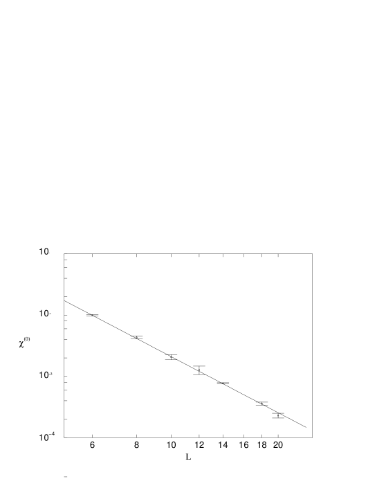
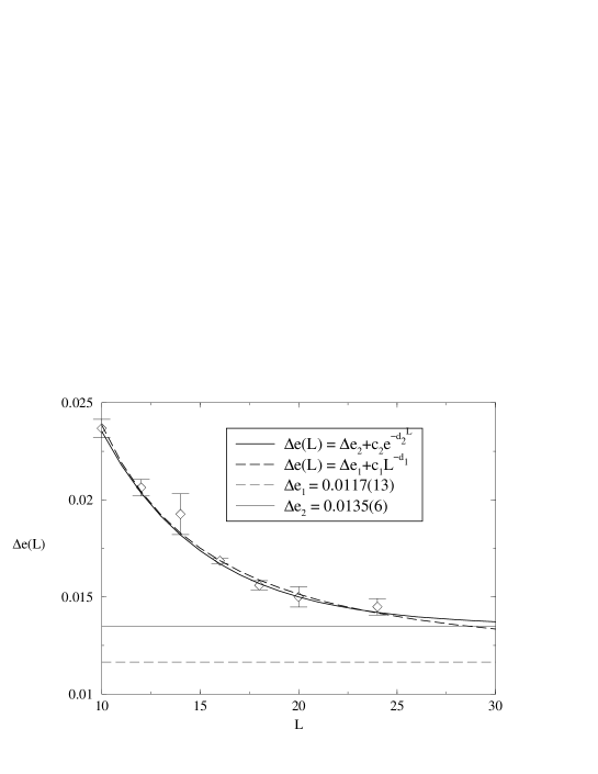
FIG. 3.: FSS of $\chi^{(0)}$, the imaginary part of the zeroes in the partition function. This is a log-log plot, so the fit must be a line (the solid line)

FIG. 4.: FSS of the latent heat. Data fit so well an exponential law (33) and a potential one (32).

V Conclusions

Among different appealing features the world-sheet formulation avoids the summation over redundant gauge configurations. This fact implies an amelioration of the convergence to the equilibrium. As a consequence, the time series generated using this approach show a high degree of “tunneling” between phases, a phenomenon that is depressed in the standard Wilson formulation.

We have observed in the simulations a standard first order behavior in several observables (autocorrelations, specific heat, latent heat) with an intermediate behavior between the first order ($\nu=0.25$) and second order Gaussian exponent ($\nu=0.5$) like other weak first order transitions. Wether or not this observed first order signature is an artifact of the topology/boundary-conditions of the lattice is an issue we will analyze in a future work.

REFERENCES

- [1] I. Campos, A. Cruz, and A. Tarancon, “A study of the phase transition in 4-d pure compact u(1) lgt on toroidal and spherical lattices,” hep-lat/9803007.
- [2] I. Campos, A. Cruz, and A. Tarancon, “First order signatures in 4-d pure compact u(1) gauge theory with toroidal and spherical topologies,” hep-lat/9711045.
- [3] B. Klaus and C. Roiesnel, “High statistics finite size scaling analysis of u(1) lattice gauge theory with wilson action,” hep-lat/9801036.
- [4] C. Roiesnel, “Finite size effects at phase transition in compact u(1) gauge theory,” Nucl. Phys. Proc. Suppl. 63 (1998) 697, hep-lat/9709081.
- [5] J. Jersak, C. B. Lang, and T. Neuhaus, “Four-dimensional pure compact u(1) gauge theory on a spherical lattice,” Phys. Rev. D54 (1996) 6909–6922, hep-lat/9606013.
- [6] M. Baig and H. Fort, “Fixed boundary conditions and phase transitions in pure gauge compact qed,” Phys. Lett. B332 (1994) 428–432, hep-lat/9406003.
- [7] T. Banks, R. Myerson, and J. Kogut, “Phase transitions in abelian lattice gauge theories,” Nucl. Phys. B129 (1977) 493.
- [8] M. Baig, H. Fort, and J. B. Kogut, “Monopole percolation in pure gauge compact qed,” Phys. Rev. D50 (1994) 5920–5923, hep-lat/9406004.
- [9] B. Lautrup and M. Nauenberg, “Phase transition in four-dimensional compact qed,” Phys. Lett. 95B (1980) 63.
- [10] G. Bhanot, “The nature of the phase transition in compact qed,” Phys. Rev. D24 (1981) 461.
- [11] J. Jersak, T. Neuhaus, and P. M. Zerwas, “U(1) lattice gauge theory near the phase transition,” Phys. Lett. 133B (1983) 103.
- [12] V. Azcoiti, G. di Carlo, and A. F. Grillo, “Towards a precise determination of the order of the phase transition in compact pure gauge qed,” Phys. Lett. B238 (1990) 355.
- [13] G. Bhanot, T. Lippert, K. Schilling, and P. Uberholz, “First order transitions and the multihistogram method,” Nucl. Phys. B378 (1992) 633–651.
- [14] R. Gambini and A. Trias, “Second quantization of the free electromagnetic field as quantum mechanics in the loop space,” Phys. Rev. D22 (1980) 1380.
- [15] R. Gambini and A. Trias, “Gauge dynamics in the c representation,” Nucl. Phys. B278 (1986) 436.
- [16] J. M. Aroca, M. Baig, and H. Fort, “The lagrangian loop representation of lattice u(1) gauge theory,” Phys. Lett. B336 (1994) 54–61, hep-th/9407170.
- [17] J. M. Aroca, M. Baig, H. Fort, and R. Siri, “Matter fields in the lagrangian loop representation: Scalar qed,” Phys. Lett. B366 (1996) 416–420, hep-th/9507124.
- [18] A. M. Polyakov, “String representations and hidden symmetries for gauge fields,” Phys. Lett. 82B (1979) 247.
- [19] A. M. Polyakov, “Gauge fields as rings of glue,” Nucl. Phys. B164 (1980) 171.
- [20] Y. M. Makeenko and A. A. Migdal, “Exact equation for the loop average in multicolor qcd,” Phys. Lett. 88B (1979) 135.
- [21] C. N. Yang, “Integral formalism for gauge fields,” Phys. Rev. Lett. 33 (1974) 445.
- [22] A. H. Guth, “Existence proof of a nonconfining phase in four-dimensional u(1) lattice gauge theory,” Phys. Rev. D21 (1980) 2291.
- [23] D. Weingarten, “A lattice field theory for interacting strings,” Phys. Lett. 90B (1980) 280.
- [24] A. D. Sokal, “Monte carlo mehtods in statistical mechanics: Foundations and new algorithms,”.
- [25] E. Marinari, “Optimized monte carlo methods,” cond-mat/9612010.
- [26] M. Bowick, P. Coddington, L. ping Han, G. Harris, and E. Marinari, “The phase diagram of fluid random surfaces with extrinsic curvature,” Nucl. Phys. B394 (1993) 791–821, hep-lat/9209020.
- [27] E. Marinari, “Complex zeros of the d = 3 ising model: Finite size scaling and critical amplitudes,” Nucl. Phys. B235 (1984) 123.
- [28] M. Falcioni, E. Marinari, M. L. Paciello, G. Parisi, and B. Taglienti, “Complex zeros in the partition function of the four- dimensional su(2) lattice gauge model,” Phys. Lett. 108B (1982) 331.