DESY 98-097
TPR-98-19
HUB-EP-98/45
Nonperturbative Renormalisation of Composite Operators in Lattice QCD

Abstract

We investigate the nonperturbative renormalisation of composite operators in lattice QCD restricting ourselves to operators that are bilinear in the quark fields. These include operators which are relevant to the calculation of moments of hadronic structure functions. The computations are based on Monte Carlo simulations using quenched Wilson fermions.

, , , , , , , ,

1 Introduction

Monte Carlo simulations of lattice QCD have evolved from spectrum calculations to more detailed investigations of hadron structure. These more advanced studies require to calculate hadronic matrix elements of composite operators. In order to compute the moments of hadronic structure functions, for example, one needs the matrix elements of composite operators appearing in the operator product expansion of the appropriate currents [1, 2, 3, 4]. In general, one has to renormalise these operators in order to obtain finite answers in the continuum limit. Furthermore, comparison with the results of phenomenological analyses usually requires the matrix elements to be given in one of the popular continuum renormalisation schemes, e.g. the $\overline{\mathrm{MS}}$ scheme. So one has to think about the conversion of the bare lattice operators to renormalised continuum operators.

Consider the special case of the operators determining the moments of hadronic structure functions. Here the renormalised continuum matrix element has to be multiplied by the corresponding Wilson coefficient to yield the desired moment, which can be measured in deep inelastic scattering experiments. Being an observable quantity it must be independent of any choices made in the renormalisation procedure. This is of course only possible, if the renormalised matrix element and the Wilson coefficient are calculated in the same scheme. In particular, the dependence on the renormalisation scale $\mu$ has to cancel between the renormalisation constant and the Wilson coefficient. Since the Wilson coefficients are usually computed in the $\overline{\mathrm{MS}}$ scheme, we have to convert our lattice operators to continuum $\overline{\mathrm{MS}}$ operators if we want to make contact with phenomenology.

One obvious possibility to calculate the necessary renormalisation factors is lattice perturbation theory. However, quite often lattice perturbation theory seems to converge rather slowly. Identifying one source of these poor convergence properties, Lepage and Mackenzie proposed as a remedy the so-called tadpole improved perturbation theory [5]. Still, lattice perturbation series rarely extend beyond the one-loop level, and hence considerable uncertainty remains.

It is therefore only natural to try a nonperturbative renormalisation by means of Monte Carlo simulations. A way how to do this was introduced in Ref. [6]. We shall present several improvements of this method and apply it to a variety of operators that are bilinear in the quark fields [7]. In particular, we study operators which are needed to calculate hadronic structure functions. Computing the $Z$ factors for a rather large range of renormalisation scales we can find out at which scales (if at all) perturbative behaviour sets in such that the multiplication with the perturbative Wilson coefficients makes sense.

In this paper we shall work only with Wilson fermions in the quenched approximation. However, an obvious next step is the use of improved fermions in order to reduce cut-off effects. Like the renormalisation of our operators, the improvement should be nonperturbative. As far as the action is concerned, there is already a lot of experience how to achieve this. But improvement of the action is not sufficient, the operators have to be improved as well. Here a good deal of work still has to be done, in particular for operators containing derivatives.

The paper is organised as follows: After introducing in Section 2 the operators to be studied we explain the method of nonperturbative renormalisation in Section 3. In the special case of the vector and axial vector currents we prefer a variant of this method because it seems to suppress lattice artifacts more efficiently. We describe it in Section 4. Perturbative formulae, which we need for comparison and for obtaining results in the $\overline{\mathrm{MS}}$ scheme, are given in Section 5. Section 6 contains some details of the numerical implementation including our momentum sources which greatly reduce the statistical noise of the data. In Section 7 we present and discuss our results. Finally, we come to our conclusions.

2 The operators

In the Euclidean continuum we should study the operators

$${\mathcal{O}}^{(q)}_{\mu_{1}\cdots\mu_{n}}=\bar{q}\gamma_{\mu_{1}}\mbox{ \parbox[b]{0.0pt}{$D$}\raisebox{7.3194pt}{$\leftrightarrow$}${}_{\!\mu_{2}}$}\cdots\mbox{ \parbox[b]{0.0pt}{$D$}\raisebox{7.3194pt}{$\leftrightarrow$}${}_{\!\mu_{n}}$}q\,,$$ (2.1)

$${\mathcal{O}}^{5(q)}_{\sigma\mu_{1}\cdots\mu_{n}}=\bar{q}\gamma_{\sigma}\gamma_{5}\mbox{ \parbox[b]{0.0pt}{$D$}\raisebox{7.3194pt}{$\leftrightarrow$}${}_{\!\mu_{1}}$}\cdots\mbox{ \parbox[b]{0.0pt}{$D$}\raisebox{7.3194pt}{$\leftrightarrow$}${}_{\!\mu_{n}}$}q$$ (2.2)

or rather O(4) irreducible multiplets with definite C-parity. In particular, we obtain twist-2 operators by symmetrising the indices and subtracting the traces. In the flavour-nonsinglet case they do not mix and are hence multiplicatively renormalisable.

Working with Wilson fermions it is straightforward to write down lattice versions of the above operators. One simply replaces the continuum covariant derivative by its lattice analogue. However, O(4) being restricted to its finite subgroup H(4) (the hypercubic group) on the lattice, the constraints imposed by space-time symmetry are less stringent than in the continuum and the possibilities for mixing increase [2, 3, 8, 9]. Guided by the H(4) classification given in Ref. [8] we have chosen the operators [4, 10, 11]

$${\mathcal{O}}_{v_{2,a}} = {\mathcal{O}}^{(q)}_{\{14\}}\,,$$ (2.3)

$${\mathcal{O}}_{v_{2,b}} = {\mathcal{O}}^{(q)}_{\{44\}}-\mbox{\small$\frac{1}{3}$}({\mathcal{O}}^{(q)}_{\{11\}}+{\mathcal{O}}^{(q)}_{\{22\}}+{\mathcal{O}}^{(q)}_{\{33\}})\,,$$ (2.4)

$${\mathcal{O}}_{v_{3}} = {\mathcal{O}}^{(q)}_{\{114\}}-{\textstyle\frac{1}{2}}({\mathcal{O}}^{(q)}_{\{224\}}+{\mathcal{O}}^{(q)}_{\{334\}})\,,$$ (2.5)

$${\mathcal{O}}_{v_{4}} = {\mathcal{O}}^{(q)}_{\{1144\}}+{\mathcal{O}}^{(q)}_{\{2233\}}-{\mathcal{O}}^{(q)}_{\{1133\}}-{\mathcal{O}}^{(q)}_{\{2244\}}\,,$$ (2.6)

$${\mathcal{O}}_{a_{1}} = {\mathcal{O}}^{5(q)}_{\{24\}}\,,$$ (2.7)

$${\mathcal{O}}_{a_{2}} = {\mathcal{O}}^{5(q)}_{\{214\}}\,,$$ (2.8)

$${\mathcal{O}}_{r_{2,a}} = {\mathcal{O}}^{5(q)}_{\{14\}}\,,$$ (2.9)

$${\mathcal{O}}_{r_{2,b}} = {\mathcal{O}}^{5(q)}_{\{44\}}-\mbox{\small$\frac{1}{3}$}({\mathcal{O}}^{5(q)}_{\{11\}}+{\mathcal{O}}^{5(q)}_{\{22\}}+{\mathcal{O}}^{5(q)}_{\{33\}})\,,$$ (2.10)

$${\mathcal{O}}_{r_{3}} = {\mathcal{O}}^{5(q)}_{\{114\}}-{\textstyle\frac{1}{2}}({\mathcal{O}}^{5(q)}_{\{224\}}+{\mathcal{O}}^{5(q)}_{\{334\}})\,.$$ (2.11)

They are labeled by the reduced hadron matrix elements which they determine. In addition, we have studied the following operators without derivatives (“currents”):

$${\mathcal{O}}^{S} = \bar{q}q\,,$$ (2.12)

$${\mathcal{O}}^{P} = \bar{q}\gamma_{5}q\,,$$ (2.13)

$${\mathcal{O}}^{V}_{\mu} = \bar{q}\gamma_{\mu}q\,,$$ (2.14)

$${\mathcal{O}}^{A}_{\mu} = \bar{q}\gamma_{\mu}\gamma_{5}q\,,$$ (2.15)

where all quark fields are taken at the same lattice point, as well as the conserved vector current

$$J_{\mu}(x) = {\textstyle\frac{1}{2}}\Big{(}\bar{q}(x+\hat{\mu})(\gamma_{\mu}+1)U^{+}(x,\mu)q(x)$$ (2.16)

$$\hskip 85.35826pt{}+\bar{q}(x)(\gamma_{\mu}-1)U(x,\mu)q(x+\hat{\mu})\Big{)}$$

with the link matrix $U(x,\mu)\in$ SU(3) representing the gauge field.

Note that the operators ${\mathcal{O}}_{v_{2,a}}$ and ${\mathcal{O}}_{v_{2,b}}$ although belonging to the same irreducible O(4) multiplet transform according to inequivalent representations of H(4). Hence their renormalisation factors calculated on the lattice have no reason to coincide. The same remark applies to ${\mathcal{O}}_{r_{2,a}}$ and ${\mathcal{O}}_{r_{2,b}}$. The operators ${\mathcal{O}}_{a_{1}}$ and ${\mathcal{O}}_{r_{2,a}}$, on the other hand, are members of the same irreducible H(4) multiplet, hence their renormalisation factors should agree also on the lattice.

Concerning the mixing properties a few remarks are in order. Mixing with operators of equal or lower dimension is excluded for the operators ${\mathcal{O}}_{v_{2,a}}$, ${\mathcal{O}}_{v_{2,b}}$, ${\mathcal{O}}_{a_{1}}$, ${\mathcal{O}}_{a_{2}}$, ${\mathcal{O}}_{r_{2,a}}$, ${\mathcal{O}}_{r_{2,b}}$, as well as for the currents. The case of the operator ${\mathcal{O}}_{v_{3}}$, for which there are two further operators with the same dimension and the same transformation behaviour, is discussed in Refs. [8, 9]. The operators ${\mathcal{O}}_{v_{4}}$, ${\mathcal{O}}_{r_{3}}$, on the other hand, could in principle mix not only with operators of the same dimension but also with an operator of one dimension less and different chiral properties. It is of the type

$$\bar{q}\sigma_{\mu\nu}\gamma_{5}\mbox{ \parbox[b]{0.0pt}{$D$}\raisebox{7.3194pt}{$\leftrightarrow$}${}_{\!\mu_{1}}$}\mbox{ \parbox[b]{0.0pt}{$D$}\raisebox{7.3194pt}{$\leftrightarrow$}${}_{\!\mu_{2}}$}\cdots\mbox{ \parbox[b]{0.0pt}{$D$}\raisebox{7.3194pt}{$\leftrightarrow$}${}_{\!\mu_{n}}$}q\,,$$ (2.17)

where $n=2$ in the case of ${\mathcal{O}}_{v_{4}}$ and $n=1$ for ${\mathcal{O}}_{r_{3}}$.

Our analysis ignores mixing completely. This seems to be justified for ${\mathcal{O}}_{v_{3}}$. Here a perturbative calculation gives a rather small mixing coefficient for one of the mixing operators [3, 9], whereas the other candidate for mixing does not appear at all in a one-loop calculation of quark matrix elements at momentum transfer zero, because its Born term vanishes in forward direction. The same is true for all operators of dimension less or equal to 6 which transform identically to ${\mathcal{O}}_{v_{4}}$: Their Born term vanishes in forward matrix elements, hence they do not show up in a one-loop calculation at vanishing momentum transfer. In the case of ${\mathcal{O}}_{r_{3}}$, however, the mixing with an operator of lower dimension is already visible at the one-loop level even in forward direction.

3 The method

Our calculation of renormalisation constants follows closely the procedure proposed by Martinelli et al. [6]. It mimics the definitions used in (continuum) perturbation theory. We work on a lattice of spacing $a$ and volume $V$ in Euclidean space. For a fixed gauge let

$$G_{\alpha\beta}(p)=\frac{a^{12}}{V}\sum_{x,y,z}{\mathrm{e}}^{-{\mathrm{i}}p\cdot(x-y)}\langle q_{\alpha}(x){\mathcal{O}}(z)\bar{q}_{\beta}(y)\rangle$$ (3.1)

denote the non-amputated quark-quark Green function with one insertion of the operator ${\mathcal{O}}$ at momentum zero. It is to be considered as a matrix in colour and Dirac space. With the quark propagator

$$S_{\alpha\beta}(p)=\frac{a^{8}}{V}\sum_{x,y}{\mathrm{e}}^{-{\mathrm{i}}p\cdot(x-y)}\langle q_{\alpha}(x)\bar{q}_{\beta}(y)\rangle$$ (3.2)

the corresponding vertex function (or amputated Green function) is given by

$$\Gamma(p)=S^{-1}(p)G(p)S^{-1}(p)\,.$$ (3.3)

Defining the renormalised vertex function by

$$\Gamma_{\mathrm{R}}(p)=Z_{q}^{-1}Z_{\mathcal{O}}\Gamma(p)$$ (3.4)

we fix the renormalisation constant $Z_{\mathcal{O}}$ by imposing the renormalisation condition

$$\mbox{\small$\frac{1}{12}$}{\rm tr}\left(\Gamma_{\mathrm{R}}(p)\Gamma_{\mathrm{Born}}(p)^{-1}\right)=1$$ (3.5)

at $p^{2}=\mu^{2}$, where $\mu$ is the renormalisation scale. So we calculate $Z_{\mathcal{O}}$ from

$$Z_{q}^{-1}Z_{\mathcal{O}}\mbox{\small$\frac{1}{12}$}{\rm tr}\left(\Gamma(p)\Gamma_{\mathrm{Born}}(p)^{-1}\right)=1$$ (3.6)

with $p^{2}=\mu^{2}$. Here $\Gamma_{\mathrm{Born}}(p)$ is the Born term in the vertex function of ${\mathcal{O}}$ computed on the lattice, and $Z_{q}$ denotes the quark field renormalisation constant. The latter can be taken as

$$Z_{q}(p)=\frac{{\rm tr}\left(-{\rm i}\sum_{\lambda}\gamma_{\lambda}\sin(ap_{\lambda})aS^{-1}(p)\right)}{12\sum_{\lambda}\sin^{2}(ap_{\lambda})}\,,$$ (3.7)

again at $p^{2}=\mu^{2}$.

If the operator under study belongs to an O(4) multiplet of dimension greater than 1, i.e. if it carries at least one space-time index, the trace in Eq. (3.6) will in general depend on the direction of $p$. So the renormalisation condition (3.5) violates O(4) covariance even in the continuum limit. In the continuum, this disease is easily cured by a suitable summation over the members of the O(4) multiplet. On the lattice, this makes sense only in the few special cases where the O(4) multiplet is irreducible also under the hypercubic group H(4), because the renormalisation constants for the different H(4) multiplets within a given O(4) multiplet will in general be different. So we have to live with this noncovariance, which, of course, should finally be compensated when we convert our results to a covariant renormalisation scheme.

The scale $\mu$ at which our renormalisation constants are defined should ideally satisfy the conditions

$$1/L^{2}\ll\Lambda^{2}_{\mathrm{QCD}}\ll\mu^{2}\ll 1/a^{2}$$ (3.8)

on a lattice with linear extent $L$. Whether in a concrete calculation these conditions may be considered as fulfilled remains to be seen.

4 A special case: vector and axial vector currents

In the special case of the vector and axial vector currents in the continuum we can distinguish between longitudinal and transverse components with respect to the momentum. One may thus define two renormalisation constants, one from the longitudinal and one from the transverse components. Denoting the vertex function of the currents generically by $J_{\mu}(p)$ we have for the vector current (the modifications required in the case of the axial vector current are obvious)

$$Z_{q}^{-1}Z_{J}^{\mathrm{long}}\mbox{\small$\frac{1}{12}$}{\rm tr}\left(\sum_{\mu}\frac{p_{\mu}}{p^{2}}\not\!{p}J_{\mu}(p)\right)=1\,,$$ (4.1)

$$Z_{q}^{-1}Z_{J}^{\mathrm{trans}}\mbox{\small$\frac{1}{12}$}{\rm tr}\left(\sum_{\mu}\left(\gamma_{\mu}-\frac{p_{\mu}}{p^{2}}\not\!{p}\right)J_{\mu}(p)\right)=3\,.$$ (4.2)

Note that these renormalisation conditions are O(4) covariant.

We try to generalise (4.2) to the lattice imposing a renormalisation condition of the form

$$Z_{q}^{-1}Z_{J}\mbox{\small$\frac{1}{12}$}{\rm tr}\left(\sum_{\mu}Q_{\mu}^{\bot}J_{\mu}(p)\right)=\mbox{\small$\frac{1}{12}$}{\rm tr}\left(\sum_{\mu}Q_{\mu}^{\bot}J_{\mu}^{\mathrm{Born}}(p)\right)=3\,,$$ (4.3)

where $Q_{\mu}^{\bot}$ is a suitable Dirac matrix and $J_{\mu}^{\mathrm{Born}}(p)$ denotes the Born term evaluated on the lattice. In the case of the conserved vector current we know that $Z_{J}=1$, hence we can calculate $Z_{q}$ from (4.3). This value is then used to determine $Z_{J}$ for the local vector and axial vector currents.

The matrix $Q_{\mu}^{\bot}$ is constructed as

$$Q_{\mu}^{\bot}=\left(J_{\mu}^{\mathrm{Born}}\right)^{-1}-Q_{\mu}^{\|}\,,$$ (4.4)

where

$$Q_{\mu}^{\|}=\frac{1}{N}\sin(ap_{\mu})\sum_{\lambda}\left(J_{\lambda}^{\mathrm{Born}}\right)^{-1}\sin(ap_{\lambda})\,.$$ (4.5)

The normalisation factor $N$ follows immediately from the condition (4.3):

$$N=\mbox{\small$\frac{1}{12}$}{\mathrm{tr}}\left[\sum_{\mu}J_{\mu}^{\mathrm{Born}}\sin(ap_{\mu})\sum_{\lambda}\left(J_{\lambda}^{\mathrm{Born}}\right)^{-1}\sin(ap_{\lambda})\right]\,.$$ (4.6)

Note that for $a\to 0$ and $J_{\mu}^{\mathrm{Born}}\to\gamma_{\mu}$ we have $N/a^{2}\to p^{2}$, and (4.3) reduces to (4.2) in the continuum limit.

In the case of the conserved vector current we find

$$J_{\mu}^{\mathrm{Born}}(p)=\gamma_{\mu}\cos(ap_{\mu})+\mathrm{i}\sin(ap_{\mu})$$ (4.7)

so that

$$N=\left(\sum_{\mu}\sin^{2}(ap_{\mu})\right)^{2}+\sum_{\mu}\sin^{2}(ap_{\mu})-\sum_{\mu}\sin^{4}(ap_{\mu})\,.$$ (4.8)

For the local vector and axial vector current we have

$$J_{\mu}^{\mathrm{Born}}=\gamma_{\mu}$$ (4.9)

and

$$J_{\mu}^{\mathrm{Born}}=\gamma_{\mu}\gamma_{5}\,,$$ (4.10)

respectively, and we obtain in both cases

$$N=\sum_{\mu}\sin^{2}(ap_{\mu})\,.$$ (4.11)

Working with the longitudinal component, i.e. with a lattice version of (4.1), leads to a less smooth momentum dependence, i.e. to stronger lattice effects.

5 Input from perturbative calculations

Eq. (3.5) defines a renormalisation scheme of the momentum subtraction type, which we call MOM scheme. Note that it will in general not agree with any of the momentum subtraction schemes used in continuum perturbation theory. It is desirable to convert our results into a more popular scheme like the $\overline{\mathrm{MS}}$ scheme. Moreover, we want to use our renormalisation factors in connection with the Wilson coefficients, which appear in the operator product expansion, and these are generally given in the $\overline{\mathrm{MS}}$ scheme. Hence we have to perform a finite renormalisation leading us from the renormalisation scheme defined by Eq. (3.5) to the $\overline{\mathrm{MS}}$ scheme. The corresponding renormalisation constant $Z^{\overline{\mathrm{MS}}}_{\mathrm{MOM}}$ is computed in continuum perturbation theory using dimensional regularisation.

We work in a general covariant gauge (gauge parameter $\xi$) such that the gluon propagator has the form

$$\frac{1}{p^{2}}\left(\delta_{\mu\nu}-(1-\xi)\frac{p_{\mu}p_{\nu}}{p^{2}}\right)\,.$$ (5.1)

The Landau gauge, which is employed in our numerical simulations, corresponds to $\xi=0$. Most of our operators can be written in the form

$$\sum_{\mu_{1},\ldots,\mu_{n}}c_{\mu_{1}\ldots\mu_{n}}\left(\bar{q}\gamma_{\{\mu_{1}}\mbox{ \parbox[b]{0.0pt}{$D$}\raisebox{7.3194pt}{$\leftrightarrow$}${}_{\!\mu_{2}}$}\cdots\mbox{ \parbox[b]{0.0pt}{$D$}\raisebox{7.3194pt}{$\leftrightarrow$}${}_{\!\mu_{n}\}}$}\gamma_{5}^{n_{5}}q-\mathrm{traces}\right)$$ (5.2)

where $n_{5}=0,1$ and $c_{\mu_{1}\ldots\mu_{n}}$ is totally symmetric and traceless. Neglecting quark masses one obtains with an anticommuting $\gamma_{5}$

$$Z^{\overline{\mathrm{MS}}}_{\mathrm{MOM}} = 1+\frac{g^{2}}{16\pi^{2}}C_{F}\Bigg{[}G_{n}+(1-\xi)S_{n-1}$$ (5.3)

$${}+\left(-\frac{4}{n+1}+(1-\xi)\frac{2}{n}\right)\frac{\left(\sum_{\mu}p_{\mu}h_{\mu}(p)\right)^{2}}{p^{2}\sum_{\mu}h_{\mu}(p)^{2}}\Bigg{]}+O(g^{4})\,,$$

where $C_{F}=4/3$ for the gauge group SU(3),

$$G_{n} = \frac{2}{n(n+1)}\left(-3-S_{n-1}+2S_{n+1}\right)$$ (5.4)

$$\hskip 85.35826pt{}+\frac{2}{n+1}-4\sum_{j=2}^{n}\frac{1}{j}\left(2S_{j}-S_{j-1}\right)-1\,,$$

$$S_{n} = \sum_{j=1}^{n}\frac{1}{j}\,,$$ (5.5)

and

$$h_{\mu}(p)=\sum_{\mu_{2},\ldots,\mu_{n}}c_{\mu\mu_{2}\ldots\mu_{n}}p_{\mu_{2}}\cdots p_{\mu_{n}}\,.$$ (5.6)

Because of the noncovariance of our renormalisation condition, $Z^{\overline{\mathrm{MS}}}_{\mathrm{MOM}}$ depends on the direction of the momentum $p$ and on the coefficients $c_{\mu_{1},\ldots,\mu_{n}}$.

For ${\mathcal{O}}^{S}$ and ${\mathcal{O}}^{P}$ we obtain

$$Z^{\overline{\mathrm{MS}}}_{\mathrm{MOM}}=1+\frac{g^{2}}{16\pi^{2}}(4+\xi)C_{F}+O(g^{4})\,.$$ (5.7)

In this special case we can go one step further and use the two-loop result for $Z^{\overline{\mathrm{MS}}}_{\mathrm{MOM}}$ [12]. For three colours and $n_{f}$ flavours one has in Landau gauge:

$$Z^{\overline{\mathrm{MS}}}_{\mathrm{MOM}}=1+\frac{16}{3}\cdot\frac{g^{2}}{16\pi^{2}}+\left(177.48452-\frac{83}{9}n_{f}\right)\left(\frac{g^{2}}{16\pi^{2}}\right)^{2}+O(g^{6})\,.$$ (5.8)

We want to compare our nonperturbative results with the corresponding values obtained in (tadpole improved) perturbation theory on the lattice. For the renormalisation factor which brings us from the bare lattice operator to the renormalised operator in the $\overline{\mathrm{MS}}$ scheme, lattice perturbation theory yields results of the form

$$Z^{\mathrm{pert}}_{\mathcal{O}}=1-\frac{g^{2}}{16\pi^{2}}(\gamma_{0}\ln(a\mu)+C_{F}\Delta_{\mathcal{O}})$$ (5.9)

where $\Delta_{\mathcal{O}}$ is a finite constant and $\gamma_{0}$ is the one-loop coefficient of the anomalous dimension. Working with an anticommuting $\gamma_{5}$ also in the continuum part of the calculation we arrive at the values given in Table 1 (see Ref. [9] for more details).

Table 1: Finite contributions to the renormalisation factors in lattice perturbation theory. In addition, the one- and two-loop coefficients of the anomalous dimension are given for 0 flavours.

${\mathcal{O}}$	$\Delta_{\mathcal{O}}$	$\gamma_{0}$	$\gamma_{1}$
${\mathcal{O}}_{v_{2,a}}$	1.2796	64/9	96.69
${\mathcal{O}}_{v_{2,b}}$	2.5619	64/9	96.69
${\mathcal{O}}_{v_{3}}$	$-12.1274$	100/9	141.78
${\mathcal{O}}_{v_{4}}$	$-27.2296$	628/45	172.58
${\mathcal{O}}_{a_{2}}$	$-12.1171$	100/9	141.78
${\mathcal{O}}_{r_{2,a}}$	0.3451	64/9	96.69
${\mathcal{O}}_{r_{2,b}}$	0.1674	64/9	96.69
${\mathcal{O}}_{r_{3}}$	$-12.8589$	100/9	141.78
${\mathcal{O}}^{S}$	12.9524	$-8$	$-134.67$
${\mathcal{O}}^{P}$	22.5954	$-8$	$-134.67$
${\mathcal{O}}^{V}_{\mu}$	20.6178	0	0.00
${\mathcal{O}}^{A}_{\mu}$	15.7963	0	0.00

In order to obtain the corresponding results in tadpole improved perturbation theory [5] we write (with $\mu=1/a$) for an operator with $n_{D}$ covariant derivatives

$$1-\frac{g^{2}}{16\pi^{2}}C_{F}\Delta_{\mathcal{O}} = \frac{u_{0}}{u_{0}^{n_{D}}}u_{0}^{n_{D}-1}\left(1-\frac{g^{2}}{16\pi^{2}}C_{F}\Delta_{\mathcal{O}}\right)$$ (5.10)

$$= \frac{u_{0}}{u_{0}^{n_{D}}}\left(1-\frac{g^{*2}}{16\pi^{2}}C_{F}\overline{\Delta}_{\mathcal{O}}\right)+O(g^{*4})\,,$$

where

$$u_{0}=\langle\mbox{\small$\frac{1}{3}$}\mathrm{tr}U_{\Box}\rangle^{\frac{1}{4}}=1-\frac{g^{2}}{16\pi^{2}}C_{F}\pi^{2}+O(g^{4})$$ (5.11)

and

$$\overline{\Delta}_{\mathcal{O}}=\Delta_{\mathcal{O}}+(n_{D}-1)\pi^{2}\,.$$ (5.12)

This reflects the fact that one has $n_{D}$ operator tadpole diagrams and one leg tadpole diagram, which are of the same magnitude but contribute with opposite sign. Furthermore, one chooses as the expansion parameter $g^{*}$ the coupling constant renormalised at some physical scale. We have taken $g^{*}$ from the values given for $\alpha_{\overline{\mathrm{MS}}}(1/a)$ in Table I of Ref. [5].

At this point we have two options. Either we stay with the expression (5.9) and its tadpole improved analogue

$$Z^{\mathrm{ti}}_{\mathcal{O}}=u_{0}^{1-n_{D}}\left[1-\frac{g^{*2}}{16\pi^{2}}(\gamma_{0}\ln(a\mu)+C_{F}\overline{\Delta}_{\mathcal{O}})\right]$$ (5.13)

or we apply these formulae only at a fixed scale $\mu=\mu_{0}$ (e.g. $\mu_{0}=1/a$) using the renormalisation group to change $\mu$.

For this scale dependence, the renormalisation group predicts (at fixed bare parameters)

$$R_{\mathcal{O}}(\mu,\mu_{0}):=\frac{Z_{\mathcal{O}}(\mu)}{Z_{\mathcal{O}}(\mu_{0})}=\exp\left\{-\int_{\bar{g}(\mu_{0}^{2})}^{\bar{g}(\mu^{2})}\mathrm{d}g\frac{\gamma(g)}{\beta(g)}\right\}\,.$$ (5.14)

Here the $\beta$-function is given by

$$\beta(g)=-\beta_{0}\frac{g^{3}}{16\pi^{2}}-\beta_{1}\frac{g^{5}}{(16\pi^{2})^{2}}+\cdots$$ (5.15)

with

$$\beta_{0}=11-\frac{2}{3}n_{f}\,,\,\beta_{1}=102-\frac{38}{3}n_{f}\,.$$ (5.16)

In terms of the $\Lambda$ parameter the running coupling reads

$$\frac{\bar{g}^{2}(\mu^{2})}{16\pi^{2}}=\frac{1}{\beta_{0}\ln(\mu^{2}/\Lambda^{2})}-\frac{\beta_{1}}{\beta_{0}^{3}}\frac{\ln\ln(\mu^{2}/\Lambda^{2})}{\ln^{2}(\mu^{2}/\Lambda^{2})}+\cdots$$ (5.17)

and the anomalous dimension is expanded as

$$\gamma(g)=\gamma_{0}\frac{g^{2}}{16\pi^{2}}+\gamma_{1}\left(\frac{g^{2}}{16\pi^{2}}\right)^{2}+\cdots$$ (5.18)

For our operators the one- and two-loop coefficients $\gamma_{0}$ and $\gamma_{1}$ of the anomalous dimension are known in the $\overline{\mathrm{MS}}$ scheme [13, 14]. The values actually used are listed in Table 1. Within the two-loop approximation we obtain

$$R_{\mathcal{O}}(\mu,\mu_{0})=\left(\frac{\bar{g}^{2}(\mu^{2})}{\bar{g}^{2}(\mu_{0}^{2})}\right)^{\frac{\gamma_{0}}{2\beta_{0}}}\left(\frac{1+\frac{\beta_{1}}{\beta_{0}}\frac{\bar{g}^{2}(\mu^{2})}{16\pi^{2}}}{1+\frac{\beta_{1}}{\beta_{0}}\frac{\bar{g}^{2}(\mu_{0}^{2})}{16\pi^{2}}}\right)^{{\textstyle\frac{1}{2}}\left((\gamma_{1}/\beta_{1})-(\gamma_{0}/\beta_{0})\right)}\,.$$ (5.19)

In the case of the operators ${\mathcal{O}}^{S}$ and ${\mathcal{O}}^{P}$ we can do better and use the three-loop expressions for the $\beta$ function and the anomalous dimension. In the $\overline{\mathrm{MS}}$ scheme one finds [15, 16, 17]

$$\beta_{2} = \frac{2857}{2}-\frac{5033}{18}n_{f}+\frac{325}{54}n_{f}^{2}\,,$$

$$\gamma_{1} = -\frac{404}{3}+\frac{40}{9}n_{f}\,,$$ (5.20)

$$\gamma_{2} = -2498+\left(\frac{4432}{27}+\frac{320}{3}\zeta_{3}\right)n_{f}+\frac{280}{81}n_{f}^{2}\,,$$

where $\zeta_{3}\approx 1.2020569032$. For the running coupling we have now instead of (5.17)

$$\frac{\bar{g}^{2}(\mu^{2})}{16\pi^{2}} = \frac{1}{\beta_{0}\ln(\mu^{2}/\Lambda^{2})}-\frac{\beta_{1}}{\beta_{0}^{3}}\frac{\ln\ln(\mu^{2}/\Lambda^{2})}{\ln^{2}(\mu^{2}/\Lambda^{2})}$$ (5.21)

$${}+\frac{1}{\beta_{0}^{5}\ln^{3}(\mu^{2}/\Lambda^{2})}\left(\beta_{1}^{2}\ln^{2}\ln(\mu^{2}/\Lambda^{2})-\beta_{1}^{2}\ln\ln(\mu^{2}/\Lambda^{2})\right.$$

$$\hskip 142.26378pt{}+\left.\beta_{2}\beta_{0}-\beta_{1}^{2}\right)+\cdots$$

and $R_{\mathcal{O}}$ takes the form

$$R_{\mathcal{O}}(\mu,\mu_{0})=\frac{\exp F\left(\frac{\bar{g}^{2}(\mu^{2})}{16\pi^{2}}\right)}{\exp F\left(\frac{\bar{g}^{2}(\mu_{0}^{2})}{16\pi^{2}}\right)}$$ (5.22)

with

$$F(x) = \frac{\gamma_{0}}{2\beta_{0}}\ln x+\frac{\beta_{0}\gamma_{2}-\beta_{2}\gamma_{0}}{4\beta_{0}\beta_{2}}\ln\left(\beta_{0}+\beta_{1}x+\beta_{2}x^{2}\right)$$ (5.23)

$${}+\frac{2\beta_{0}\beta_{2}\gamma_{1}-\beta_{1}\beta_{2}\gamma_{0}-\beta_{0}\beta_{1}\gamma_{2}}{2\beta_{0}\beta_{2}\sqrt{4\beta_{0}\beta_{2}-\beta_{1}^{2}}}\arctan\left(\frac{\beta_{1}+2\beta_{2}x}{\sqrt{4\beta_{0}\beta_{2}-\beta_{1}^{2}}}\right)\,.$$

Having data at two different values of the bare coupling we can also compare the dependence on the bare coupling with the behaviour expected from the renormalisation group. Keeping the renormalisation scale $\mu$ and the renormalised quantities fixed we find for the ratio of the renormalisation factors $Z_{\mathcal{O}}$ and $Z_{\mathcal{O}}^{\prime}$ at the bare couplings $g$ and $g^{\prime}$, respectively,

$$\frac{Z_{\mathcal{O}}}{Z_{\mathcal{O}}^{\prime}}=\exp\left\{\int_{g^{\prime}}^{g}\mathrm{d}g_{0}\frac{\hat{\gamma}(g_{0})}{\hat{\beta}(g_{0})}\right\}\,.$$ (5.24)

Here $\hat{\gamma}(g)$ and $\hat{\beta}(g)$ denote the anomalous dimension and the $\beta$-function obtained by differentiation with respect to the cut-off at fixed renormalised quantities. They are considered as functions of the bare coupling. Within the two-loop approximation we get

$$\frac{Z_{\mathcal{O}}}{Z_{\mathcal{O}}^{\prime}}=\left(\frac{g^{2}}{g^{\prime 2}}\right)^{-\frac{\gamma_{0}}{2\beta_{0}}}\left(\frac{1+\frac{\beta_{1}}{\beta_{0}}\frac{g^{2}}{16\pi^{2}}}{1+\frac{\beta_{1}}{\beta_{0}}\frac{g^{\prime 2}}{16\pi^{2}}}\right)^{-{\textstyle\frac{1}{2}}\left((\hat{\gamma}_{1}/\beta_{1})-(\gamma_{0}/\beta_{0})\right)}\,,$$ (5.25)

where we have used the fact that $\beta_{0}$, $\beta_{1}$, and $\gamma_{0}$ are universal so that $\hat{\beta}_{0}=\beta_{0}$, $\hat{\beta}_{1}=\beta_{1}$, $\hat{\gamma}_{0}=\gamma_{0}$. The coefficient $\hat{\gamma}_{1}$ reads (cf. also [18])

$$\hat{\gamma}_{1}=\gamma_{1}+2\beta_{0}C_{F}\Delta_{\mathcal{O}}-32\pi^{2}\gamma_{0}\left(-0.234101+n_{f}\cdot 0.0034435\right)$$ (5.26)

for the gauge group SU(3). The quantities $\Delta_{\mathcal{O}}$ are given in Table 1, and the coefficient of $\gamma_{0}$ stems from the ratio of the $\Lambda$-parameters on the lattice and in the $\overline{\mathrm{MS}}$ scheme (see, e.g., [19]).

6 Numerical implementation

Let us sketch the main ingredients of our calculational procedure. To simplify the notation we set the lattice spacing $a=1$ in this section. In a first step gauge field configurations are generated and numerically fixed to some convenient gauge (the Landau gauge in our case). The non-amputated Green function (3.1) is calculated as the gauge field average of $\hat{G}(p)$, which is constructed from the quark propagator $\hat{S}(p)$ on the same gauge field configuration according to

$$\hat{G}(p)=\frac{1}{V}\sum_{x,y,z,z^{\prime}}{\mathrm{e}}^{-{\mathrm{i}}p\cdot(x-y)}\hat{S}(x,z)J(z,z^{\prime})\hat{S}(z^{\prime},y)\,.$$ (6.1)

We omit the quark-line disconnected contribution (which would contribute only to flavour-singlet operators) and suppress Dirac as well as colour indices. The operator under study is represented by $J(z,z^{\prime})$:

$$\sum_{z}{\mathcal{O}}(z)=\sum_{z,z^{\prime}}\bar{q}(z)J(z,z^{\prime})q(z^{\prime})\,.$$ (6.2)

Using the relation

$$\hat{S}(x,y)=\gamma_{5}\hat{S}(y,x)^{+}\gamma_{5}$$ (6.3)

we rewrite $\hat{G}(p)$ as

$$\hat{G}(p)=\sum_{z,z^{\prime}}\gamma_{5}\left(\sum_{x}\hat{S}(z,x){\mathrm{e}}^{{\mathrm{i}}p\cdot x}\right)^{+}\gamma_{5}J(z,z^{\prime})\left(\sum_{y}\hat{S}(z^{\prime},y){\mathrm{e}}^{{\mathrm{i}}p\cdot y}\right)$$ (6.4)

in terms of the quantities

$$\sum_{x}\hat{S}(z,x){\mathrm{e}}^{{\mathrm{i}}p\cdot x}\,.$$ (6.5)

These can be calculated by solving the lattice Dirac equation with a momentum source:

$$\sum_{z}M(y,z)\left(\sum_{x}\hat{S}(z,x){\mathrm{e}}^{{\mathrm{i}}p\cdot x}\right)={\mathrm{e}}^{{\mathrm{i}}p\cdot y}\,.$$ (6.6)

Here $M(x,y)$ represents the fermion matrix. So the number of matrix inversions to be performed is proportional to the number of momenta considered. But the quark propagators, which we need for the amputation and the computation of the quark wave function renormalisation, are immediately obtained from the quantities already calculated.

Another computational strategy would be to choose a particular location for the operator, i.e. instead of summing over $z^{\prime}$ (and $z$) in (6.1) one could set $z^{\prime}=0$. Translational invariance tells us that this will give the same expectation value after averaging over all gauge field configurations. For this method we need to solve the Dirac equation with a point source at the location of the operator and (in the case of extended operators) for a small number of point sources in the immediate neighbourhood. For operators with a small number of derivatives the point source method would require fewer inversions, but it turns out that relying on translational invariance leads to much larger statistical errors. This is clearly seen in the results shown in Ref. [20], which were obtained with a point source instead of a momentum source (cf. also Ref. [21]).

We work with standard Wilson fermions ($r=1$) in the quenched approximation. At $\beta=6.0$ we have analysed 20 configurations on a $16^{3}\times 32$ lattice for three values of the hopping parameter, $\kappa=0.155$, 0.153, and 0.1515. Four further configurations at $\beta=6.2$ on a $24^{3}\times 48$ lattice were studied with $\kappa=0.152$, 0.1507, and 0.1489. For the critical $\kappa$ we take the values $\kappa_{c}=0.157211$ ($\beta=6.0$) and $\kappa_{c}=0.153374$ ($\beta=6.2$), respectively (see Ref. [22]).

Before we calculate quark correlation functions on our configurations we fix the gauge to the Landau gauge [23]. The gauge fixing necessarily raises the question of the influence of Gribov copies. Fortunately, an investigation of this problem in a similar setting indicates that the fluctuations induced by the Gribov copies are not overwhelmingly large and may be less important than the ordinary statistical fluctuations [24]. Therefore we decided to neglect the Gribov problem for the time being, but a careful study in the case at hand is certainly desirable.

Coming finally to the choice of the momenta, we tried to avoid momenta along the coordinate axes in order to minimise cut-off effects. Altogether we used 43 momenta at $\beta=6.0$ and 41 momenta at $\beta=6.2$.

7 Results

For the presentation of our results we convert lattice units to physical units using $a^{-2}=3.8$ GeV² ($\beta=6.0$) and $a^{-2}=7.0$ GeV² ($\beta=6.2$) as determined from the string tension [22]. This leads to values for the spatial extent of our lattices of 1.6 fm ($\beta=6.0$) and 1.8 fm ($\beta=6.2$). The $\Lambda$ parameter is taken to be $\Lambda_{\overline{\mathrm{MS}}}=230$ MeV. This value follows from the result given in Ref. [25] by using the string tension instead of the force parameter $r_{0}$ to set the scale. As we work in the quenched approximation we have to put $n_{f}=0$ in the perturbative formulae. The plotted errors are purely statistical and have been calculated by a jackknife procedure.

The quark masses used in our simulations are rather large. On the other hand, the perturbative calculations, which we use for comparison and for converting to the $\overline{\mathrm{MS}}$ scheme, are performed at vanishing quark mass. Hence we first extrapolate our results to the chiral limit. This is done linearly in $1/\kappa$. In most cases the mass dependence is quite weak so that the extrapolation looks reliable, see Fig. 1 for an example (operator ${\mathcal{O}}_{v_{2,a}}$ at $\beta=6.2$). This is not too surprising since the mass scale in the calculations is not set by the quark mass, but by the (off-shell) momentum, which is typically much larger. The only exception is the pseudoscalar density where a rather strong mass dependence is found. This observation already indicates that the pseudoscalar density is something special, and we will discuss this operator in more detail in Subsection 7.2.

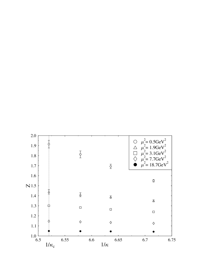
Figure 1: Chiral extrapolation of $Z$ for ${\mathcal{O}}_{v_{2,a}}$ at $\beta=6.2$. Some representative values of $\mu^{2}$ have been selected.

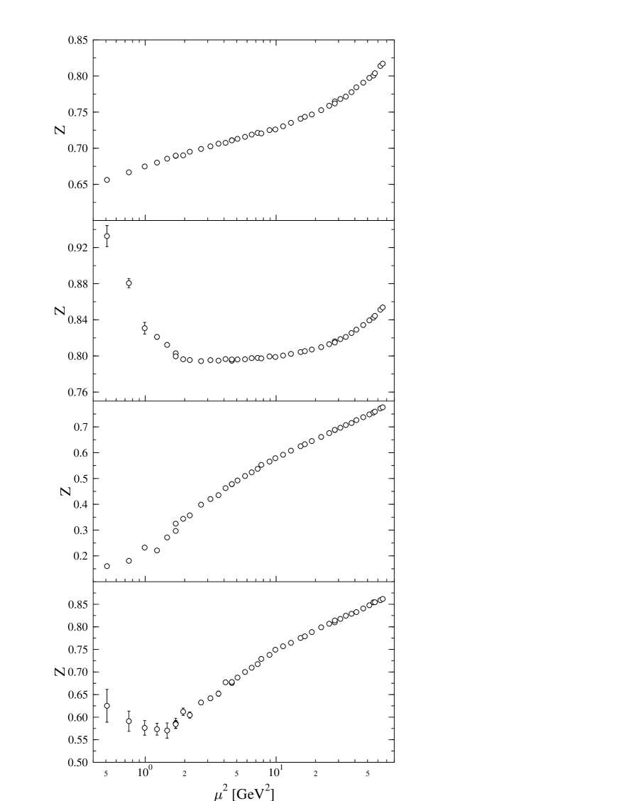
Figure 2: $Z$ in the MOM scheme for ${\mathcal{O}}^{V}_{\mu}$, ${\mathcal{O}}^{A}_{\mu}$, ${\mathcal{O}}^{P}$, and ${\mathcal{O}}^{S}$ (from top to bottom) at $\beta=6.2$. For the local vector current and the axial vector current, $Z$ has been determined from the transverse components (cf. Section 4).

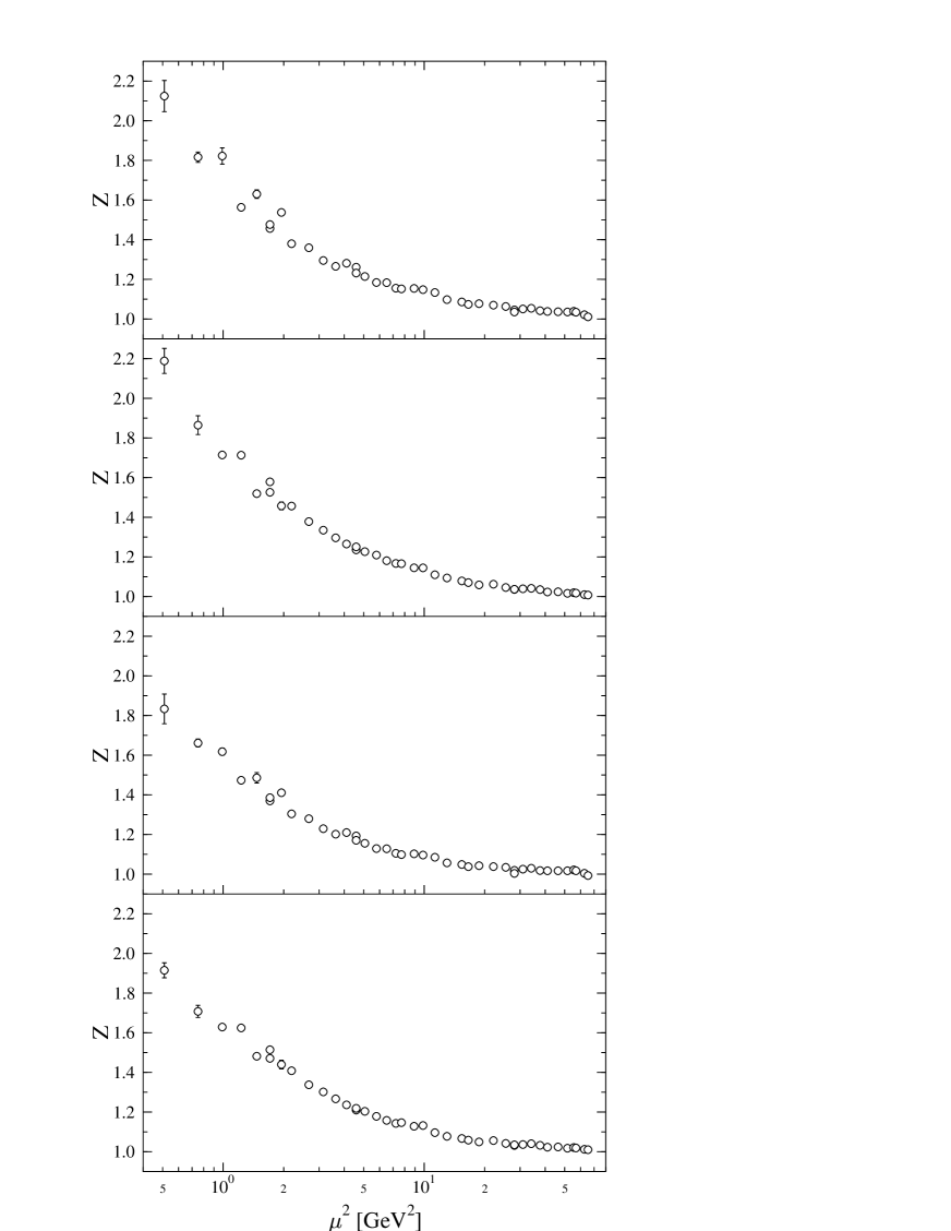
Figure 3: $Z$ in the MOM scheme for ${\mathcal{O}}_{r_{2,b}}$, ${\mathcal{O}}_{r_{2,a}}$, ${\mathcal{O}}_{v_{2,b}}$, and ${\mathcal{O}}_{v_{2,a}}$ (from top to bottom) at $\beta=6.2$.

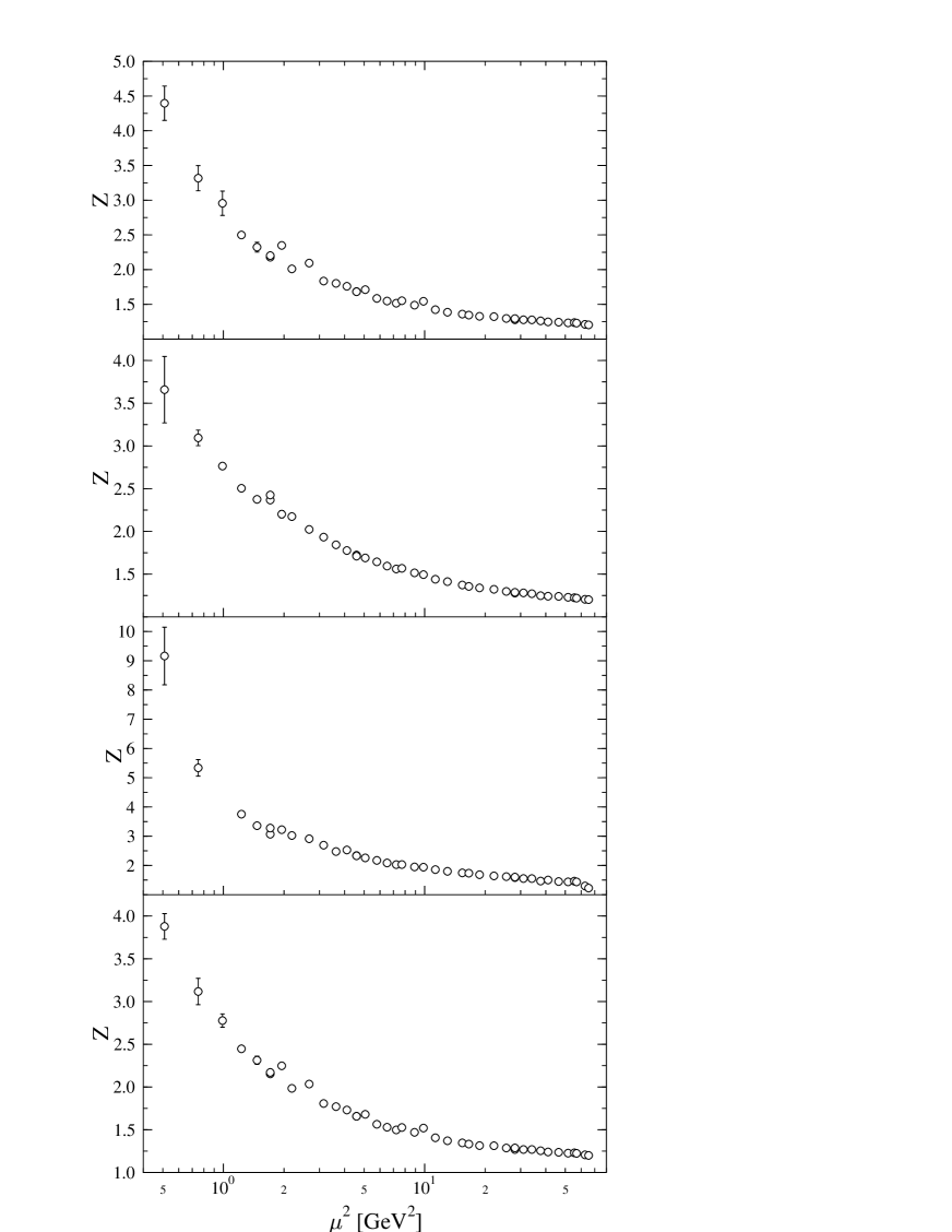
Figure 4: $Z$ in the MOM scheme for ${\mathcal{O}}_{r_{3}}$, ${\mathcal{O}}_{a_{2}}$, ${\mathcal{O}}_{v_{4}}$, and ${\mathcal{O}}_{v_{3}}$ (from top to bottom) at $\beta=6.2$.

In Figs. 2 - 4 we display our “raw” results, i.e. the nonperturbative $Z$’s in our MOM scheme, for $\beta=6.2$. Then we multiply by $Z^{\overline{\mathrm{MS}}}_{\mathrm{MOM}}$ in order to obtain the $Z$ factors in the $\overline{\mathrm{MS}}$ scheme. When evaluating the perturbative expression for $Z^{\overline{\mathrm{MS}}}_{\mathrm{MOM}}$ we insert for the coupling constant the running coupling in the $\overline{\mathrm{MS}}$ scheme taken at the renormalisation scale $\mu^{2}$ (cf. Eq. (5.17)). Fig. 5 illustrates the effect of the conversion to the $\overline{\mathrm{MS}}$ scheme for the operator ${\mathcal{O}}_{v_{2,a}}$ at $\beta=6.2$.

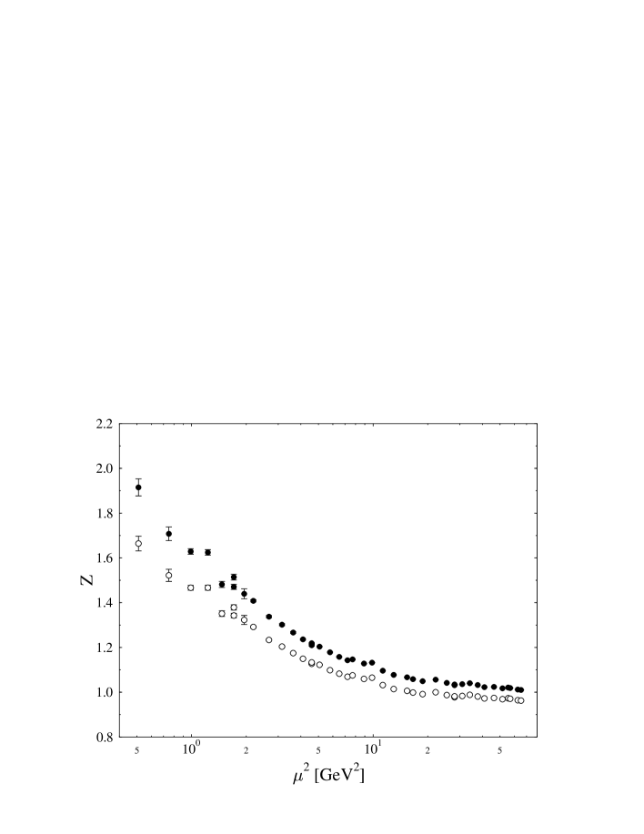
Figure 5: $Z$ for the operator ${\mathcal{O}}_{v_{2,a}}$ at $\beta=6.2$. The filled circles represent the data corresponding to the MOM renormalisation condition (3.5), the open circles represent the values in the $\overline{\mathrm{MS}}$ scheme.

Ultimately we are interested in physical observables, e.g. in the moments of the structure functions. They are obtained from the bare matrix elements calculated on the lattice after multiplication by the appropriate $Z$ factor and the Wilson coefficient (both computed in the $\overline{\mathrm{MS}}$ scheme). So the bridge from the lattice to continuum physics consists of the product of these two quantities. Having calculated $Z$ nonperturbatively we can multiply with the corresponding Wilson coefficient in order to see if the expected cancellation of the $\mu$ dependence really occurs. If it does, the $\mu$ independent value of the product is the factor we need in order to calculate the moments of the structure functions from the lattice results. Since this cancellation means that the scale dependence of our $Z$’s should be described by the renormalisation group factor $R$ (given by (5.19) in two-loop approximation) we shall divide our numerical results by this expression and define $Z_{\mathrm{RGI}}=Z/R$. For $Z_{\mathrm{RGI}}$ we hope to obtain a $\mu$ independent answer, at least in a reasonable window of $\mu$ values. We shall choose $\mu_{0}^{2}=4$ GeV² in (5.19).

7.1 Vector and axial vector currents

Let us begin with the vector and axial vector currents. Since in these cases the $\overline{\mathrm{MS}}$ anomalous dimensions vanish, the renormalisation group factor (5.19) equals 1 and we expect to find immediately scale independent results in a suitable window. As already mentioned, the standard procedure from Section 3 suffers more strongly from lattice artifacts than the alternative method described in Section 4. This is exemplified in Fig. 6. The results obtained by applying the standard procedure to $\bar{q}\gamma_{4}\gamma_{5}q$ scatter more strongly than the $Z$’s from the transverse component of the axial vector current. In the remainder of this paper we shall only use the values delivered by the latter procedure.

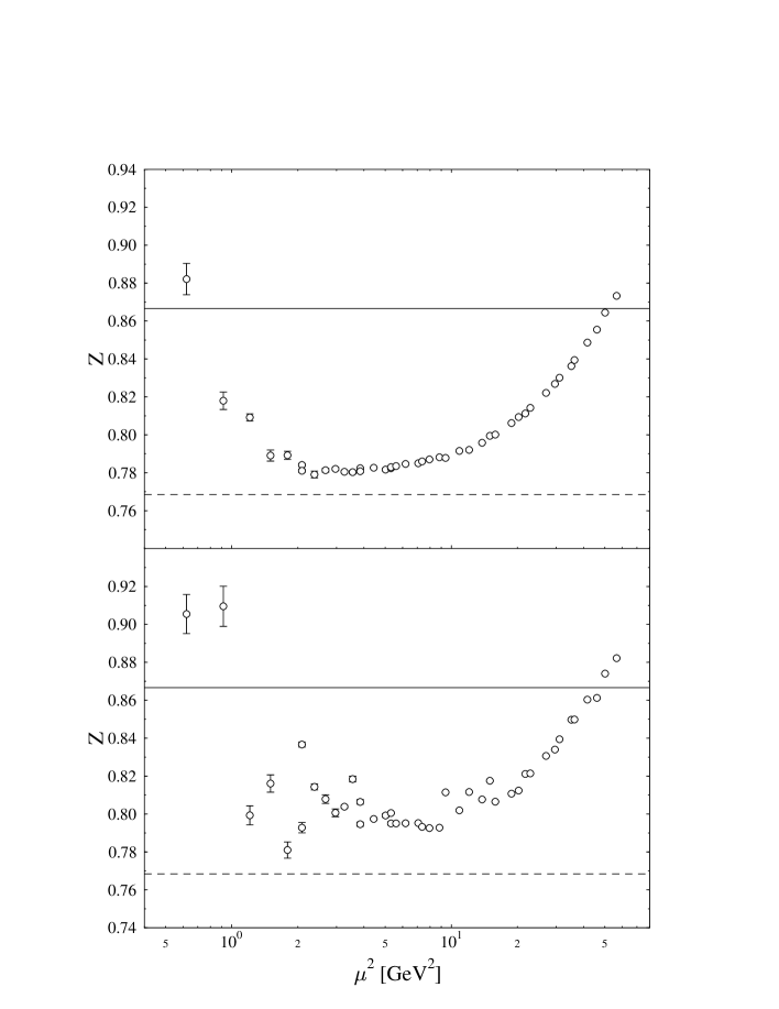
Figure 6: $Z$ for the axial vector current (transverse component) at $\beta=6.0$ determined by the method of Section 4 (upper plot). The lower plot shows $Z$ for the operator $\bar{q}\gamma_{4}\gamma_{5}q$ at the same $\beta$ value. The dashed (solid) line represents the prediction of one-loop lattice perturbation theory with (without) tadpole improvement.

Fig. 6 nicely fulfills our expectations. We see a flat region around $\mu^{2}\approx 4$ GeV² where $Z$ becomes scale independent as it should. Moreover, tadpole improvement has really improved the agreement between our nonperturbative result and one-loop lattice perturbation theory.

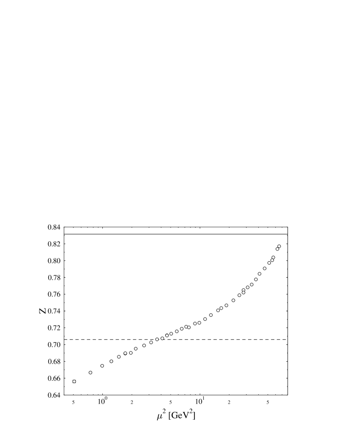
Figure 7: $Z$ for the local vector current (transverse component) at $\beta=6.2$ determined by the method of Section 4. The dashed (solid) line represents the prediction of one-loop lattice perturbation theory with (without) tadpole improvement.

The analogous plot for the transverse component of the local vector current is displayed in Fig. 7. No indication of a scaling window is seen. How can this different behaviour of local vector and axial vector current be explained? A hint may be obtained from lattice perturbation theory. If one keeps all terms of order $am$ one gets an additional contribution of the qualitatively correct form in the case of the local vector current, whereas the analogous contribution to the renormalisation of the axial vector current is considerably smaller [26]. Due to the spontaneous breakdown of chiral symmetry one should expect that some mass-like effects survive even in the chiral limit and may lead to the observed behaviour of the local vector current through such $am$ terms.

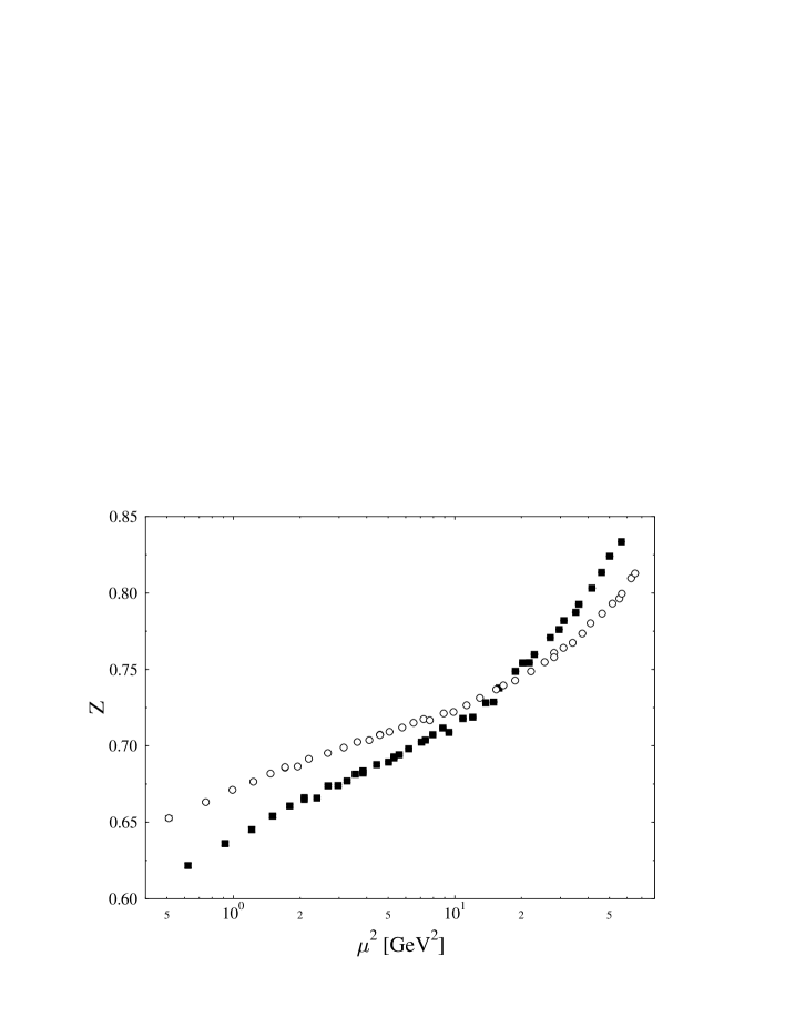
Figure 8: $Z$ for the local vector current (transverse component). The open circles (filled squares) represent the data for $\beta=6.2$ ($\beta=6.0$). The $\beta=6.2$ data have been rescaled perturbatively to $\beta=6.0$ by multiplication with (5.25).

This interpretation is supported by a comparison of the data at $\beta=6.0$ and $\beta=6.2$. The perturbative renormalisation group tells us that the $\beta$ dependence of the $Z$’s is given by the $\mu^{2}$ independent factor (5.25) in terms of the bare coupling constants $g$ and $g^{\prime}$. Therefore we multiply the $\beta=6.2$ data with the factor (5.25) and plot them together with the $Z$’s at $\beta=6.0$ versus the renormalisation scale $\mu^{2}$. The results are shown in Fig. 8 for the local vector current and in Fig. 9 for the axial vector current. In both cases, the $\beta=6.2$ data are closer to our expectations, but the local vector current seems to be more sensitive to the variation of $a$ than the axial current, in accord with the above mentioned stronger influence of $am$ corrections in lattice perturbation theory. Indeed, comparing the slopes of the data for the local vector current at the two $\beta$ values in the region below $\mu^{2}\approx 15$ GeV² one can estimate a ratio of about 1.45, close to the ratio $a(\beta=6.0)/a(\beta=6.2)\approx 1.36$.

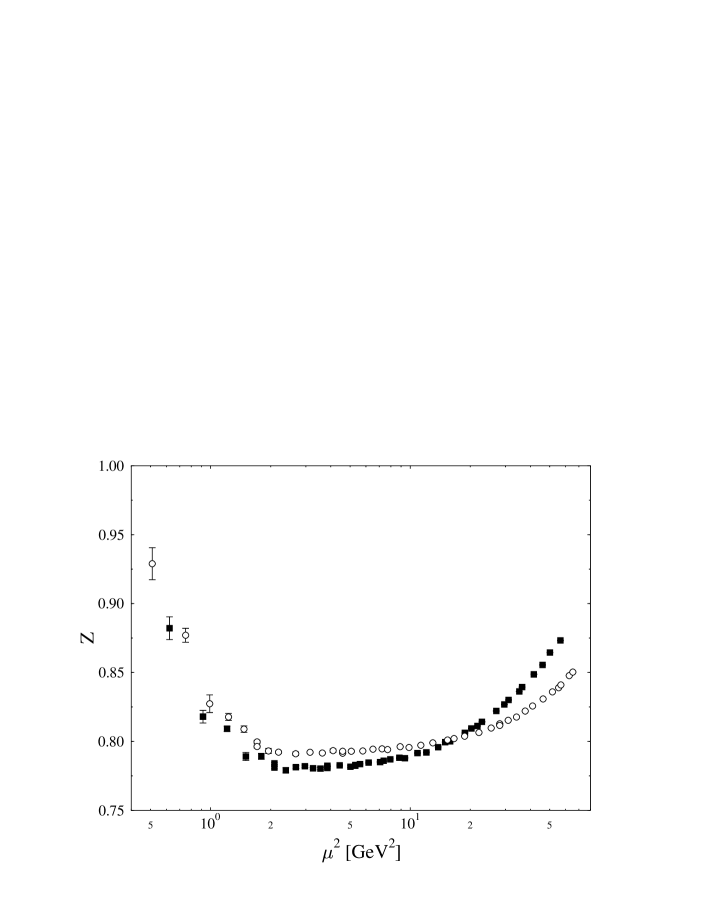
Figure 9: $Z$ for the axial vector current (transverse component). The open circles (filled squares) represent the data for $\beta=6.2$ ($\beta=6.0$). The $\beta=6.2$ data have been rescaled perturbatively to $\beta=6.0$ by multiplication with (5.25).

7.2 Scalar and pseudoscalar density

Fig. 10 shows our results for the $Z$ factor of the scalar density. The upper part of the figure compares the nonperturbative numbers transformed to the $\overline{\mathrm{MS}}$ scheme with the predictions from lattice perturbation theory with and without tadpole improvement. We also display the curves resulting from renormalisation group improvement applied to the perturbative results at $\mu_{0}^{2}=4$ GeV². Tadpole improvement works in the right direction and the data seem to follow the trend required by the renormalisation group if $\mu^{2}$ is not too small. This is more clearly exhibited in the lower part of the figure where we have divided by the renormalisation group factor (5.19). As expected, we find a nice scaling window in $Z_{\mathrm{RGI}}$ although some lattice artifacts are clearly visible.

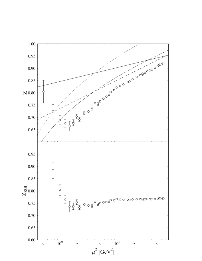
Figure 10: $Z$ and $Z_{\mathrm{RGI}}$ for the scalar density at $\beta=6.2$. The dashed (solid) straight line represents the prediction of one-loop lattice perturbation theory with (without) tadpole improvement (Eqs. (5.13), (5.9), respectively). The dotted curve results from improving the perturbative prediction with the renormalisation group (cf. Eq. (5.14)) and matching at $\mu_{0}^{2}=4$ GeV². The dash-dotted curve represents the same modification for tadpole improved perturbation theory.

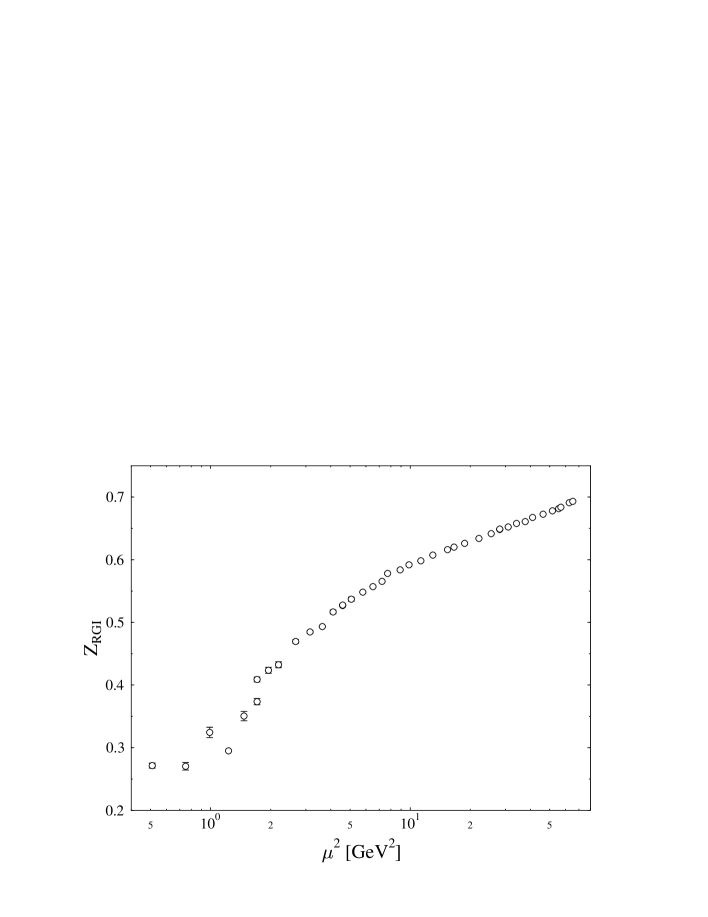
Figure 11: $Z_{\mathrm{RGI}}$ for the pseudoscalar density at $\beta=6.2$.

The results for the pseudoscalar density do not agree with the naive expectation that $Z_{\mathrm{RGI}}$ should be constant (see Fig. 11). This observation was already made by Martinelli et al.[6]. Moreover the data show a strong mass dependence, especially for the lower values of $\mu^{2}$. These features can be explained by the dynamics of chiral symmetry breaking [6]. Indeed, in the continuum there is a Ward identity relating the (bare) pseudoscalar vertex $\Gamma^{P}(p)$ at momentum transfer zero to the quark propagator:

$$-2m_{0}\Gamma^{P}(p)=S^{-1}(p)\gamma_{5}+\gamma_{5}S^{-1}(p)\,.$$ (7.1)

Here $m_{0}$ is the bare quark mass, which is taken to be nonzero. According to Pagels [27], spontaneous breakdown of chiral symmetry produces a mass-like contribution to $S^{-1}$ which commutes (rather than anticommutes) with $\gamma_{5}$ and persists in the chiral limit. Thus the r.h.s. of (7.1) will not vanish for $m_{0}\to 0$ and the pseudoscalar vertex must diverge. Consequently, the pseudoscalar density is ill defined if the chiral limit is performed after the momentum transfer has been set to zero, which is the order of limits in our procedure.

For our $Z$ factors the identity (7.1) would lead to

$$Z_{{\mathcal{O}}^{P}}(p)=-\frac{12m_{0}Z_{q}(p)}{\mathrm{tr}S^{-1}(p)}$$ (7.2)

and with $\mathrm{tr}S^{-1}(p)$ remaining nonzero even in the chiral limit $Z_{{\mathcal{O}}^{P}}(p)$ should vanish for $m_{0}\to 0$. This tendency is indeed shown by our data (at least for the lower values of $\mu^{2}$).

Nevertheless, for sufficiently large $\mu^{2}$, i.e. in the perturbative regime, the ratio $Z_{{\mathcal{O}}^{P}}/Z_{{\mathcal{O}}^{S}}$ should become constant, because ${\mathcal{O}}^{P}$ and ${\mathcal{O}}^{S}$ have equal anomalous dimensions. Comparison of the lower part of Fig. 10 with Fig. 11 shows that our data do not display this behaviour. The ratio continues to rise up to our largest values of $\mu^{2}$.

7.3 Operators with derivatives

In this subsection we want to discuss some selected operators with derivatives, which determine moments of hadronic structure functions. Again, we would like to find a “window” at moderate values of $\mu^{2}$ where $Z_{\mathrm{RGI}}$ is constant. There $\mu^{2}$ would be large enough to allow for perturbative scaling behaviour and the multiplication with perturbative Wilson coefficients would make sense. On the other hand, $\mu^{2}$ should be small enough to avoid strong cut-off effects. Indeed, as we have seen, the results for the scalar density are rather close to this ideal scenario. For operators with derivatives the situation is however less favourable.

Looking at the results for $Z_{\mathrm{RGI}}$ one observes that one gets similar values for all operators containing the same number $n_{D}$ of derivatives. They increase with $n_{D}$. Qualitatively, this behaviour is reproduced by lattice perturbation theory, and tadpole improvement enhances the effect, though not in quantitative agreement with the nonperturbative data. In order to facilitate the comparison of the different operators we have chosen the same vertical scale in the plots for all operators with the same number of derivatives although in some cases this has the consequence that the results for a few low values of $\mu^{2}$ do not appear on the plot.

Figure 12: $Z_{\mathrm{RGI}}$ for ${\mathcal{O}}_{v_{2,a}}$ at $\beta=6.2$.

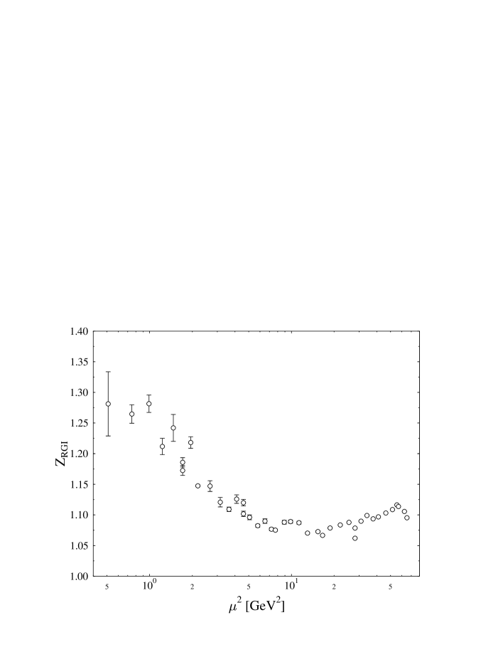
Figure 13: $Z_{\mathrm{RGI}}$ for ${\mathcal{O}}_{v_{2,b}}$ at $\beta=6.2$.

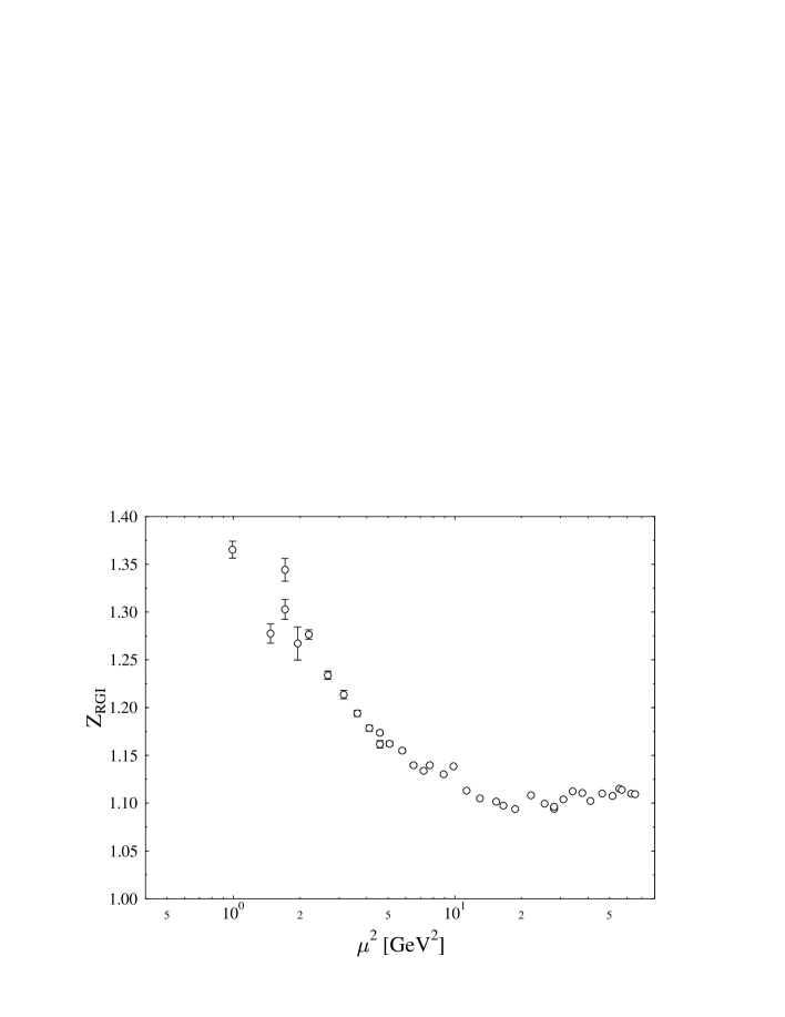
Figure 14: $Z_{\mathrm{RGI}}$ for ${\mathcal{O}}_{r_{2,a}}$ at $\beta=6.2$.

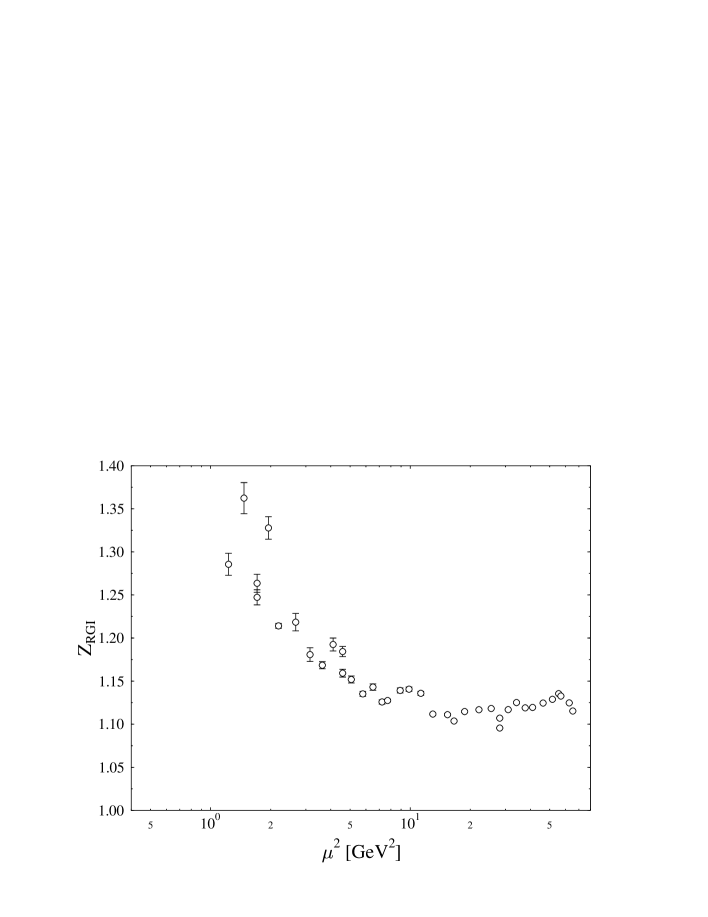
Figure 15: $Z_{\mathrm{RGI}}$ for ${\mathcal{O}}_{r_{2,b}}$ at $\beta=6.2$.

In Figs. 12-15 we plot $Z_{\mathrm{RGI}}$ versus the renormalisation scale $\mu^{2}$ for various operators containing one derivative. In most cases, a “flat” region starts only at $\mu^{2}\approx 10$ GeV², where it is hard to believe that cut-off effects are negligible. Only for ${\mathcal{O}}_{v_{2,b}}$ (may be also for ${\mathcal{O}}_{r_{2,b}}$) the window might extend to lower $\mu^{2}$. It should also be noted that for larger values of $\mu^{2}$ the scale dependence of $Z$ itself (and of $R$) is already rather weak so that approximate independence of $\mu^{2}$ is relatively easy to get. Let us now compare operators belonging to the same O(4) representation in the continuum but transforming differently under H(4) on the lattice so that their lattice $Z$’s may be different although their continuum $Z$’s must coincide. Remember that we have two pairs of that kind: ${\mathcal{O}}_{v_{2,a}}$, ${\mathcal{O}}_{v_{2,b}}$ and ${\mathcal{O}}_{r_{2,a}}$, ${\mathcal{O}}_{r_{2,b}}$. The results for ${\mathcal{O}}_{v_{2,a}}$ lie consistently above those for ${\mathcal{O}}_{v_{2,b}}$, whereas the separation between ${\mathcal{O}}_{r_{2,a}}$ and ${\mathcal{O}}_{r_{2,b}}$ is less clear. Having an anticipatory look at Table 5 below we note that one-loop lattice perturbation theory predicts the observed ordering in the case of ${\mathcal{O}}_{v_{2,a}}$, ${\mathcal{O}}_{v_{2,b}}$ although it underestimates the size of the difference. For ${\mathcal{O}}_{r_{2,a}}$, ${\mathcal{O}}_{r_{2,b}}$, on the other hand, it predicts a splitting which is roughly one order of magnitude smaller than in the previous case.

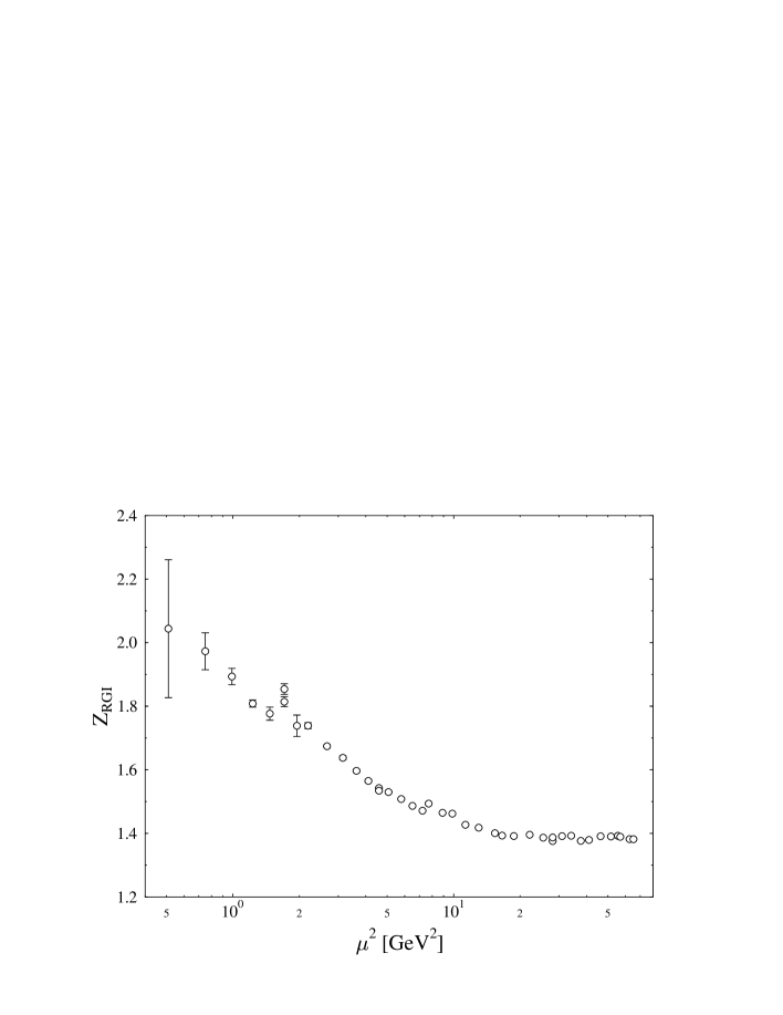
Figure 16: $Z_{\mathrm{RGI}}$ for ${\mathcal{O}}_{a_{2}}$ at $\beta=6.2$.

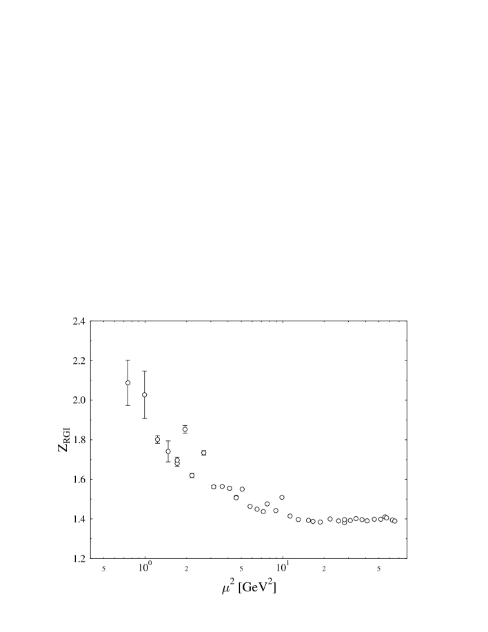
Figure 17: $Z_{\mathrm{RGI}}$ for ${\mathcal{O}}_{r_{3}}$ at $\beta=6.2$.

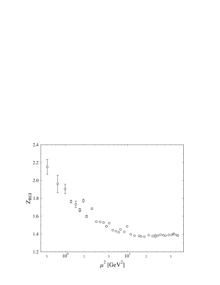
Figure 18: $Z_{\mathrm{RGI}}$ for ${\mathcal{O}}_{v_{3}}$ at $\beta=6.2$.

In Figs. 16-18 we plot $Z_{\mathrm{RGI}}$ versus the renormalisation scale $\mu^{2}$ for three operators containing two derivatives. The size of the numbers as well as their spread is larger than in the case of the operators with only one derivative. Again, a flat region is observed only for rather large values of $\mu^{2}$. One should also keep in mind that potential mixing problems in the case of ${\mathcal{O}}_{r_{3}}$ and ${\mathcal{O}}_{v_{3}}$ have been neglected.

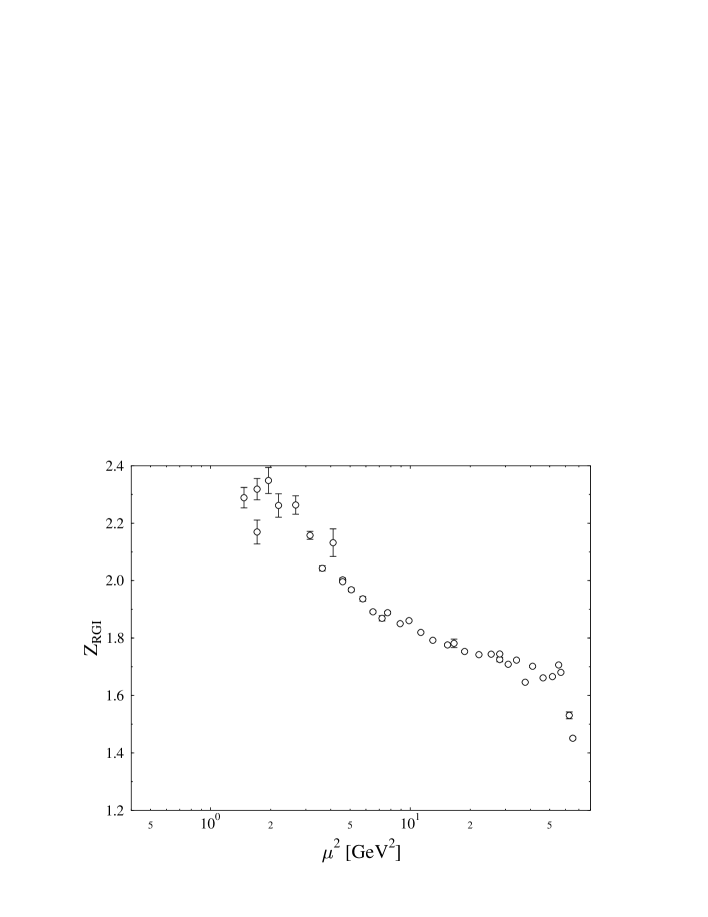
Figure 19: $Z_{\mathrm{RGI}}$ for ${\mathcal{O}}_{v_{4}}$ at $\beta=6.2$.

In the case of ${\mathcal{O}}_{v_{4}}$, an operator with three derivatives, it is simply impossible to identify a scaling window as Fig. 19 shows. This could be due to the neglected mixing problems (cf. Section 2). If this is true, the scaling behaviour should be a sensitive test of any attempt to take the mixing into account. But one would expect anyhow that cut-off effects might be relatively strong because of the large extent of the lattice operator.

7.4 Comparing $\beta=6.0$ and $\beta=6.2$

Let us now compare our results at $\beta=6.0$ and $\beta=6.2$ for a few representative operators. According to the perturbative renormalisation group, the ratio of the $Z$’s is given by the $\mu^{2}$ independent factor (5.25) in terms of the bare coupling constants $g$ and $g^{\prime}$. In Figs. 20-23 we plot $Z_{\mathrm{RGI}}$ for $\beta=6.0$ and for $\beta=6.2$ versus the renormalisation scale $\mu^{2}$. The corresponding plots for the local vector and axial vector currents have already been shown in Figs. 8 and 9. The $\beta=6.2$ data have been rescaled by multiplication with (5.25), which indeed moves them closer to the $\beta=6.0$ results. Even outside the scaling windows, the $\beta$ dependence of our data seems to be compatible with the perturbative expectation (5.25), at least for most of our operators. At first sight, this is somewhat puzzling: The perturbative renormalisation group seems to describe the dependence on the bare coupling better than the dependence on the momentum scale $\mu$. However, the ratio $a^{2}(\beta=6.0)/a^{2}(\beta=6.2)\approx 1.84=1.36^{2}$ is not terribly large and the factor (5.25) differs from one by at most 2 - 3 %. Therefore this test of the $\beta$ dependence is not too stringent.

Figure 20: $Z_{\mathrm{RGI}}$ for ${\mathcal{O}}^{S}$. The open circles (filled squares) represent the data for $\beta=6.2$ ($\beta=6.0$). The $\beta=6.2$ data have been rescaled perturbatively to $\beta=6.0$ by multiplication with (5.25).

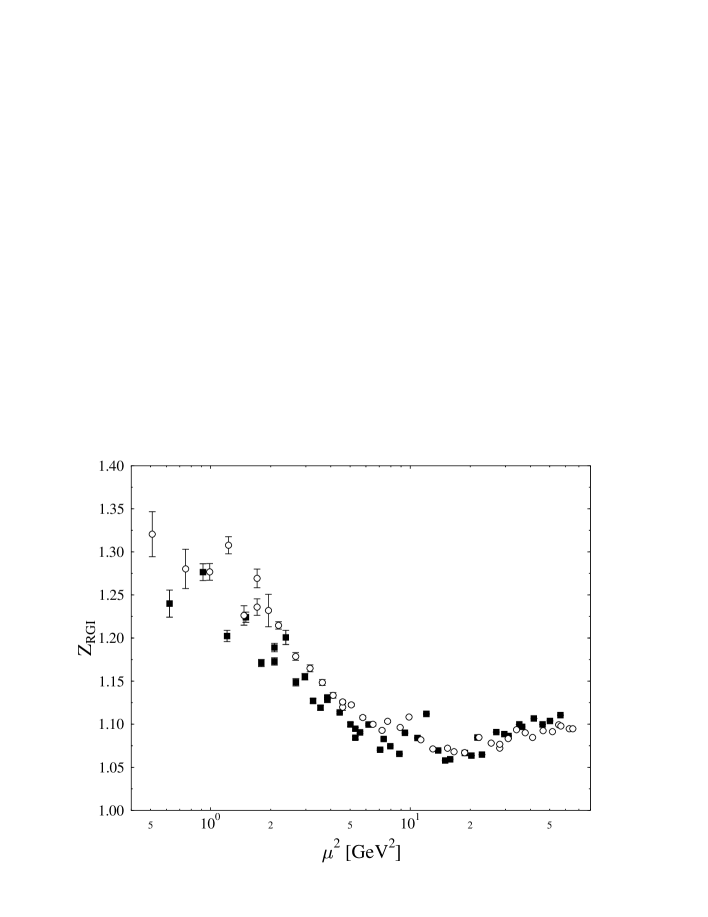
Figure 21: The same as Fig. 20, but for ${\mathcal{O}}_{v_{2,a}}$.

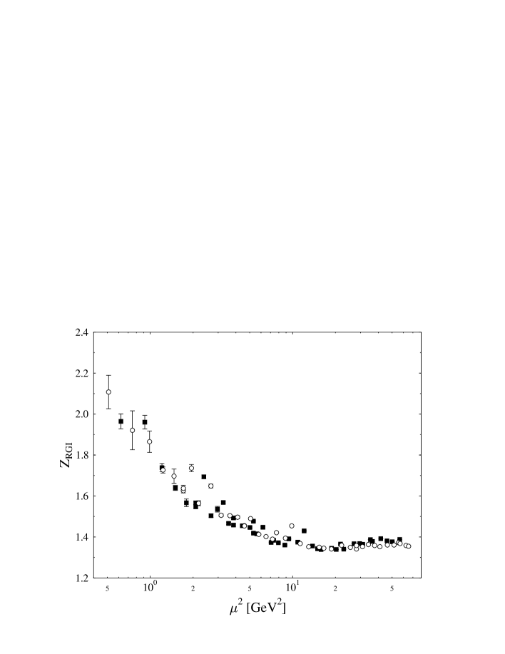
Figure 22: The same as Fig. 20, but for ${\mathcal{O}}_{v_{3}}$.

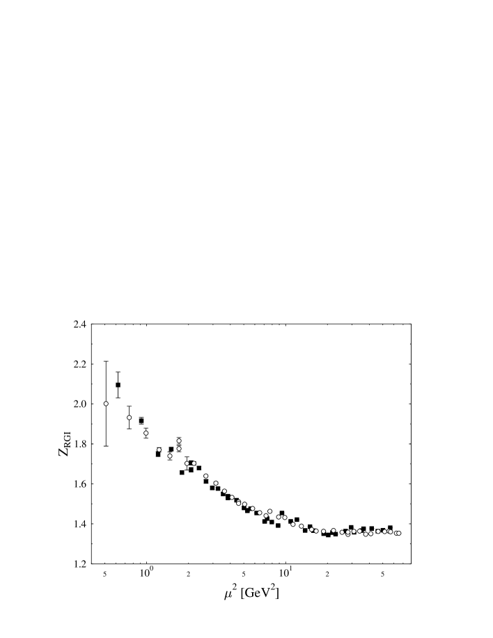
Figure 23: The same as Fig. 20, but for ${\mathcal{O}}_{a_{2}}$.

Still, it is remarkable that the $\beta$ dependence is close to perturbative even for rather small values of $\mu^{2}$. This may be taken as an indication that the observed $\mu^{2}$ dependence is a real physical effect even in regions where it does not follow the perturbative renormalisation group.

Table 2: Renormalisation factors in the MOM scheme at selected values of the renormalisation scale $\mu^{2}a^{2}$ in lattice units. The errors are purely statistical.

$\beta$	$\mu^{2}a^{2}$	${\mathcal{O}}^{A}_{\mu}$	${\mathcal{O}}^{V}_{\mu}$	${\mathcal{O}}^{P}$	${\mathcal{O}}^{S}$
	0.318	0.809(2)	0.645(2)	0.229(3)	0.602(9)
	0.626	0.779(2)	0.6658(6)	0.360(3)	0.658(4)
	0.935	0.7803(9)	0.6814(8)	0.431(2)	0.679(1)
	1.320	0.7816(7)	0.6893(7)	0.487(1)	0.720(1)
6.0	1.860	0.7850(4)	0.7024(6)	0.5347(7)	0.742(1)
	2.477	0.7878(4)	0.7088(5)	0.5772(5)	0.7752(4)
	3.942	0.7995(2)	0.7286(3)	0.6320(2)	0.8041(2)
	5.330	0.8094(2)	0.7543(3)	0.6731(2)	0.8100(2)
	7.797	0.8268(2)	0.7761(3)	0.7127(2)	0.8352(2)
	0.313	0.7954(8)	0.6951(3)	0.357(4)	0.605(7)
	0.587	0.797(1)	0.7075(3)	0.463(3)	0.6772(9)
	0.930	0.7976(4)	0.7189(3)	0.524(1)	0.709(3)
	1.272	0.7994(4)	0.7251(3)	0.566(1)	0.738(2)
6.2	1.855	0.8022(4)	0.7352(2)	0.6078(9)	0.7646(8)
	2.369	0.8053(2)	0.7435(1)	0.6328(4)	0.7790(7)
	4.014	0.8161(1)	0.7649(1)	0.6877(3)	0.8100(4)
	5.385	0.8254(1)	0.77760(9)	0.7150(1)	0.8289(2)
	7.921	0.84238(8)	0.80054(5)	0.75556(5)	0.8542(2)

Table 3: Renormalisation factors in the MOM scheme at selected values of the renormalisation scale $\mu^{2}a^{2}$ in lattice units. The errors are purely statistical.

$\beta$	$\mu^{2}a^{2}$	${\mathcal{O}}_{v_{2,a}}$	${\mathcal{O}}_{v_{2,b}}$	${\mathcal{O}}_{v_{3}}$	${\mathcal{O}}_{v_{4}}$
	0.318	1.467(8)	1.430(9)	2.42(3)	5.7(1.3)
	0.626	1.352(9)	1.294(9)	2.08(1)	2.94(2)
	0.935	1.219(3)	1.160(3)	1.692(7)	2.44(1)
	1.320	1.162(2)	1.139(3)	1.596(3)	2.31(2)
6.0	1.860	1.1042(9)	1.069(1)	1.454(2)	2.000(4)
	2.477	1.0999(7)	1.0486(5)	1.431(2)	1.879(8)
	3.942	1.0366(4)	1.0527(8)	1.3167(9)	1.701(3)
	5.330	1.0254(2)	1.0094(2)	1.2753(5)	1.64(1)
	7.797	1.0271(2)	1.0107(2)	1.2615(4)	0.909(2)
	0.313	1.408(5)	1.304(2)	1.98(2)	3.02(5)
	0.587	1.236(3)	1.210(7)	1.731(8)	2.53(6)
	0.930	1.158(2)	1.128(4)	1.529(2)	2.084(5)
	1.272	1.128(1)	1.102(3)	1.4696(6)	1.950(3)
6.2	1.855	1.0774(7)	1.057(2)	1.3709(5)	1.799(3)
	2.369	1.0583(5)	1.038(1)	1.3319(4)	1.73(1)
	4.014	1.0313(2)	1.0190(7)	1.2680(4)	1.583(7)
	5.385	1.0321(2)	1.0181(5)	1.2543(3)	1.466(2)
	7.921	1.0210(2)	1.0211(4)	1.2296(5)	1.463(1)

Table 4: Renormalisation factors in the MOM scheme at selected values of the renormalisation scale $\mu^{2}a^{2}$ in lattice units. The errors are purely statistical.

$\beta$	$\mu^{2}a^{2}$	${\mathcal{O}}_{a_{2}}$	${\mathcal{O}}_{r_{2,a}}$	${\mathcal{O}}_{r_{2,b}}$	${\mathcal{O}}_{r_{3}}$
	0.318	2.44(2)	1.539(5)	1.60(1)	2.52(3)
	0.626	2.06(1)	1.382(7)	1.417(10)	2.19(1)
	0.935	1.796(7)	1.259(4)	1.235(3)	1.724(7)
	1.320	1.636(5)	1.189(3)	1.211(3)	1.629(4)
6.0	1.860	1.503(3)	1.129(1)	1.1230(9)	1.478(2)
	2.477	1.494(3)	1.1162(7)	1.1040(5)	1.455(2)
	3.942	1.360(1)	1.0458(4)	1.0942(8)	1.331(1)
	5.330	1.2852(6)	1.0282(2)	1.0387(3)	1.2869(6)
	7.797	1.2773(6)	1.0308(2)	1.0363(2)	1.2710(5)
	0.313	2.17(1)	1.457(6)	1.380(3)	2.01(1)
	0.587	1.776(5)	1.265(3)	1.281(8)	1.760(8)
	0.930	1.594(2)	1.181(2)	1.183(4)	1.548(2)
	1.272	1.5152(8)	1.145(1)	1.154(3)	1.4884(8)
6.2	1.855	1.4124(5)	1.0938(9)	1.098(1)	1.3869(5)
	2.369	1.3564(3)	1.0704(6)	1.0737(10)	1.3455(4)
	4.014	1.2782(3)	1.0358(3)	1.0460(6)	1.2780(3)
	5.385	1.2479(3)	1.0351(2)	1.0417(4)	1.2627(3)
	7.921	1.2241(3)	1.0194(2)	1.0386(3)	1.2372(4)

Table 5: Renormalisation factors in the $\overline{\mathrm{MS}}$ scheme for $\beta=6.0$ at $\mu^{2}=a^{-2}=3.8$ GeV² and for $\beta=6.2$ at $\mu^{2}=a^{-2}=7$ GeV² .The errors of the nonperturbative values $Z_{\mathcal{O}}$ are purely statistical.

${\mathcal{O}}$		$Z_{\mathcal{O}}$	$Z^{\mathrm{ti}}_{\mathcal{O}}$	$Z^{\mathrm{pert}}_{\mathcal{O}}$		$Z_{\mathcal{O}}$	$Z^{\mathrm{ti}}_{\mathcal{O}}$	$Z^{\mathrm{pert}}_{\mathcal{O}}$
		$\beta=6.0$				$\beta=6.2$
${\mathcal{O}}_{v_{2,a}}$		1.1332(29)	0.9731	0.9892		1.0732(19)	0.9759	0.9895
${\mathcal{O}}_{v_{2,b}}$		1.0836(24)	0.9462	0.9784		1.0426(36)	0.9518	0.9791
${\mathcal{O}}_{v_{3}}$		1.4973(67)	1.1933	1.1024		1.3458(15)	1.1778	1.0991
${\mathcal{O}}_{v_{4}}$		2.0042(121)	1.5021	1.2299		1.7497(85)	1.4565	1.2225
${\mathcal{O}}_{a_{2}}$		1.5409(64)	1.1930	1.1023		1.3962(16)	1.1776	1.0990
${\mathcal{O}}_{r_{2,a}}$		1.1615(33)	0.9927	0.9971		1.0956(18)	0.9935	0.9972
${\mathcal{O}}_{r_{2,b}}$		1.1541(24)	0.9965	0.9986		1.0912(36)	0.9968	0.9986
${\mathcal{O}}_{r_{3}}$		1.5292(68)	1.2108	1.1086		1.3628(15)	1.1934	1.1051
${\mathcal{O}}^{S}$		0.7718(16)	0.8209	0.8906		0.7897(29)	0.8337	0.8942
${\mathcal{O}}^{P}$		0.4934(24)	0.6430	0.8092		0.5888(15)	0.6731	0.8154
${\mathcal{O}}^{V}_{\mu}$		0.6833(8)	0.6795	0.8259		0.7206(3)	0.7060	0.8315
${\mathcal{O}}^{A}_{\mu}$		0.7821(9)	0.7684	0.8666		0.7978(4)	0.7864	0.8709

7.5 Compilation of results

In Tables 2 - 4 we present our results for $Z_{{\mathcal{O}}}$ in the MOM scheme at selected values of the renormalisation scale. It is to be expected that the systematic uncertainties (in particular cut-off effects) are considerably larger than the quoted statistical errors. A reasonable measure for the size of the cut-off effects might be the width of the band of data points which is typically of the order of a few percent for not too small values of $\mu^{2}$.

In Table 5 we give the nonperturbative values for $Z_{\mathcal{O}}$ in the $\overline{\mathrm{MS}}$ scheme together with $Z^{\mathrm{ti}}_{\mathcal{O}}$ and $Z^{\mathrm{pert}}_{\mathcal{O}}$ for $\mu^{2}=a^{-2}$. In order to determine the nonperturbative $Z_{\mathcal{O}}$’s for this value of $\mu^{2}$ we have interpolated linearly in $\ln\mu^{2}$ between the two neighbouring results. The given error is the larger of the two statistical errors. Disregarding the results at other values of $\mu^{2}$ we see that, with the exception of the operators containing one covariant derivative, tadpole improvement works in the right direction. In the case of the local vector and axial vector currents it even overshoots somewhat. However, only in these latter cases the improvement is quantitatively satisfactory.

The renormalisation factors for the operators without derivatives (${\mathcal{O}}^{S}$, ${\mathcal{O}}^{P}$, ${\mathcal{O}}^{V}_{\mu}$, ${\mathcal{O}}^{A}_{\mu}$) have been calculated with similar nonperturbative methods by other groups, too. However, most of these studies use either an improved fermionic action or work at different values of $\beta$ so that a direct comparison is impossible. We are aware of only one other paper dealing with Wilson fermions at $\beta=6.0$ and $\beta=6.2$ [28]. Let us compare our results as given in Table 2 with Table 3 of Ref. [28].

• In the case of the local vector and axial vector currents we find some discrepancies, which, however, decrease with increasing $\mu^{2}$. At $\beta=6.2$ we obtain consistent results for the larger values of $\mu^{2}$. The deviations could be due to the fact that we use only the transverse components of the currents. Indeed, averaging over the four $Z$’s determined from the four components of the local vector current by the method of Section 3, we arrive at Fig. 24, where also the results of Ref. [28] are shown. We observe satisfactory agreement as well as a relatively large spread of the data, which is not present in our method based on the transverse components (see Fig. 8).

• The pseudoscalar density shows a different behaviour. Our $Z$’s are consistently smaller for $\beta=6.0$, but always larger for $\beta=6.2$ (although the differences are not large). Here the chiral extrapolation might be responsible for the discrepancies. Especially for the lower values of $\mu^{2}a^{2}$ we observe deviations from a linear $1/\kappa$ dependence, which make the extrapolation somewhat questionable and ambiguous.

• For the scalar density we find satisfactory agreement if $\mu^{2}a^{2}$ is not too small. Like in our data, the ratio $Z_{{\mathcal{O}}^{P}}/Z_{{\mathcal{O}}^{S}}$ does not become constant even for the largest values of $\mu^{2}$ considered in [28].

In all cases one should keep in mind that the lattice used in [28] at $\beta=6.2$ is smaller than ours. Furthermore, the momenta may differ in direction even if they are close in length, hence part of the differences could also be lattice artifacts.

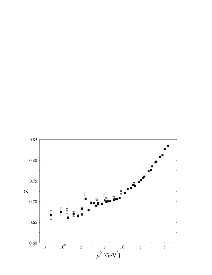
Figure 24: $Z$ for the local vector current at $\beta=6.0$. The filled squares represent our data averaged over the four components of the current. The open squares are results taken from Ref. [28].

The renormalisation constant of the local vector current can also be computed from its correlation functions with hadron sources by comparing with the corresponding correlation functions of the conserved vector current, whose renormalisation constant is known to be one. A collection of results obtained with various versions of this method at $\beta=6.0$ is given by Sachrajda [29] (cf. also [30]), albeit without extrapolation to the chiral limit. Since the quark mass dependence is rather mild, we may nevertheless compare with our numbers as displayed in Fig. 8. The values given in Ref. [29] cluster around 0.73 (computed from three-point functions) and 0.57 (computed from two-point functions). Sachrajda attributes this large difference to discretization effects. This is in accordance with our interpretation of the strong scale dependence of the $Z$ for the local vector current (see Subsection 7.1). More recently, the JLQCD collaboration has applied this method with Wilson fermions at $\beta=5.9$, 6.1, and 6.3 [31]. Interpolating their results [32] one finds 0.57 at $\beta=6.0$ and 0.62 at $\beta=6.2$.

The renormalisation of the local vector current and the axial vector current can also be studied by means of the Ward identity method [33]. However, the values obtained for Wilson fermions at $\beta=6.0$ by Maiani and Martinelli [30] (0.79(4) for the vector current and 0.85(7) for the axial vector current) refer to point-split lattice currents and are therefore not immediately comparable with our numbers. On the other hand, for the ratio $Z_{{\mathcal{O}}^{V}_{\mu}}/Z_{{\mathcal{O}}^{A}_{\mu}}$ of the renormalisation constants of the local currents they give the values 0.85(5) and 0.79(5) which are lower than (though not completely incompatible with) our result of 0.87 obtained at $\mu^{2}a^{2}=1$. From the $Z$’s which the JLQCD collaboration has calculated for the axial vector current by the Ward identity method at $\beta=5.9$, 6.1, and 6.3 one gets by interpolation [32] approximately 0.75 ($\beta=6.0$) and 0.77 ($\beta=6.2$), which is somewhat lower than our values for $\mu^{2}a^{2}=1$.

There have been various proposals to increase the accuracy in the determination of renormalisation constants, in particular by using modified versions of tadpole improvement. For $Z_{{\mathcal{O}}^{V}_{\mu}}$, $Z_{{\mathcal{O}}^{A}_{\mu}}$, and the ratio $Z_{{\mathcal{O}}^{P}}/Z_{{\mathcal{O}}^{S}}$ these are discussed in Ref. [34], where also a comparison with results from the Ward identity method is given.

8 Conclusions

We have presented a comprehensive study of nonperturbative renormalisation for various operators in the framework of lattice QCD. In particular, twist-2 operators appearing in unpolarised (polarised) deep-inelastic scattering have been studied for all spins $\leq 4$ ($\leq 3$). We worked with standard Wilson fermions at two different lattice spacings. Due to the use of momentum sources we achieved a high statistical accuracy so that systematic uncertainties (cut-off effects, in particular) are clearly visible. In order to make contact with perturbation theory one would like to identify scaling windows where the renormalisation scale $\mu$ is large enough to make perturbation theory trustworthy but small enough to allow to neglect cut-off effects. In this respect some operators did not follow our (naive) expectations. Whereas the axial vector current and the scalar density behave as expected, the local vector current and the pseudoscalar density do not show perturbative scaling. A second thought, however, revealed that there might be good reasons for this behaviour related to the spontaneous breakdown of chiral symmetry and there is nothing fundamentally wrong.

On the other hand, the operators containing one or more covariant derivatives seem to approach perturbative scaling only for rather large values of the renormalisation scale where cut-off effects might influence the results. Can we understand these deviations from perturbative scaling which seem to persist up to $\mu^{2}\approx 10$GeV²? If the observed scaling with $\beta$ is not only an artifact of our two $\beta$ values being relatively close to each other, the deviations from scaling in $\mu$ should be interpreted as real physics, though in a finite volume. (Recall that our lattices at the two $\beta$ values have roughly the same physical size.) So one possibility would be finite-size effects, although the experience with other observables suggests that they should be small. But genuinely nonperturbative effects cannot be ruled out, and one might also think of renormalons. In any case, one does not feel very comfortable when combining these nonperturbative $Z$’s with perturbative Wilson coefficients using a scale of, say, $\mu^{2}=4$GeV².

One remedy would be a nonperturbative calculation of the Wilson coefficients. But one can also try to reach larger values of $\mu^{2}$. In order to avoid strong cut-off effects one would then have to work at smaller lattice spacings, i.e. at $\beta>6.2$. However, this raises a new problem. At present, we have been careful to work with lattice sizes $L$ large enough that we believe finite-size effects are not serious. But if we try to reach much smaller $a$’s it soon becomes impossibly expensive to keep the physical lattice size sufficiently large. So we need a reliable method of measuring $Z$ nonperturbatively, even when finite-size effects are not negligible. Such a scheme has been suggested in Ref. [35]. The key point is to note that although the Green functions depend on $L$, the renormalisation constants do not. This means that we can nonperturbatively measure the ratios of $Z$’s at different lattice spacings by looking at the ratios of the corresponding bare Green functions, both measured on lattices of the same physical size, and with bare masses chosen so that the renormalised mass is the same in both cases. Note that to apply this scheme, we need good knowledge of the lattice spacing as a function of $\beta$, which may be a problem.

Further improvement could come from continuum perturbation theory. In the case of the scalar density the use of the two-loop formula for $Z^{\overline{\mathrm{MS}}}_{\mathrm{MOM}}$ and of the three-loop anomalous dimension improves the (approximate) scale independence of $Z_{\mathrm{RGI}}$. For the operators with derivatives we only have the two-loop anomalous dimension and a one-loop calculation of $Z^{\overline{\mathrm{MS}}}_{\mathrm{MOM}}$. Recently, however, first steps towards a three-loop computation of the anomalous dimension have been undertaken [36]. From the results already obtained, a two-loop expression for $Z^{\overline{\mathrm{MS}}}_{\mathrm{MOM}}$ can be extracted, unfortunately only in the Feynman gauge, whereas we would need the Landau gauge.

References

- [1] G. Martinelli and C.T. Sachrajda, Nucl. Phys. B306 (1988) 865; Nucl. Phys. B316 (1989) 355.
- [2] S. Capitani and G. Rossi, Nucl. Phys. B433 (1995) 351.
- [3] G. Beccarini, M. Bianchi, S. Capitani and G. Rossi, Nucl. Phys. B456 (1995) 271.
- [4] M. Göckeler, R. Horsley, E.-M. Ilgenfritz, H. Perlt, P. Rakow, G. Schierholz and A. Schiller, Phys. Rev. D53 (1996) 2317.
- [5] G.P. Lepage and P.B. Mackenzie, Phys. Rev. D48 (1993) 2250.
- [6] G. Martinelli, C. Pittori, C.T. Sachrajda, M. Testa and A. Vladikas, Nucl. Phys. B445 (1995) 81.
- [7] H. Oelrich, Thesis (Hamburg, 1998).
- [8] M. Göckeler, R. Horsley, E.-M. Ilgenfritz, H. Perlt, P. Rakow, G. Schierholz and A. Schiller, Phys. Rev. D54 (1996) 5705.
- [9] M. Göckeler, R. Horsley, E.-M. Ilgenfritz, H. Perlt, P. Rakow, G. Schierholz and A. Schiller, Nucl. Phys. B472 (1996) 309.
- [10] C. Best, M. Göckeler, R. Horsley, E.-M. Ilgenfritz, H. Perlt, P. Rakow, A. Schäfer, G. Schierholz, A. Schiller and S. Schramm, Phys. Rev. D56 (1997) 2743.
- [11] M. Göckeler, R. Horsley, L. Mankiewicz, H. Perlt, P. Rakow, G. Schierholz and A. Schiller, Phys. Lett. B414 (1997) 340.
- [12] E. Franco and V. Lubicz, Preprint ROME1-1198/98 (hep-ph/9803491).
- [13] E.G. Floratos, D.A. Ross and C.T. Sachrajda, Nucl. Phys. B129 (1977) 66; ibid. 139 (1978) 545 (E).
- [14] D.V. Nanopoulos and D.A. Ross, Nucl. Phys. B157 (1979) 273; R. Tarrach, Nucl. Phys. B183 (1981) 384.
- [15] T. van Ritbergen, J.A.M. Vermaseren and S.A. Larin, Phys. Lett. B400 (1997) 379.
- [16] J.A.M. Vermaseren, S.A. Larin and T. van Ritbergen, Phys. Lett. B405 (1997) 327.
- [17] K.G. Chetyrkin, Phys. Lett. B404 (1997) 161.
- [18] B. Alles and E. Vicari, Phys. Lett. B268 (1991) 241.
- [19] I. Montvay and G. Münster, Quantum Fields on a Lattice (Cambridge University Press, Cambridge (UK), 1994).
- [20] M. Göckeler, R. Horsley, E.-M. Ilgenfritz, H. Oelrich, H. Perlt, P. Rakow, G. Schierholz and A. Schiller, Nucl. Phys. B (Proc. Suppl.) 47 (1996) 493.
- [21] M. Göckeler, R. Horsley, H. Oelrich, H. Perlt, P. Rakow, G. Schierholz and A. Schiller, Nucl. Phys. B (Proc. Suppl.) 63 (1998) 868.
- [22] M. Göckeler, R. Horsley, H. Perlt, P. Rakow, G. Schierholz, A. Schiller and P. Stephenson, Phys. Rev. D57 (1998) 5562.
- [23] J.E. Mandula and M. Ogilvie, Phys. Lett. B185 (1987) 127.
- [24] M.L. Paciello, S. Petrarca, B. Taglienti and A. Vladikas, Phys. Lett. B341 (1994) 187.
- [25] S. Capitani, M. Guagnelli, M. Lüscher, S. Sint, R. Sommer, P. Weisz and H. Wittig, Nucl. Phys. B (Proc. Suppl.) 63 (1998) 153.
- [26] S. Capitani, M. Göckeler, R. Horsley, H. Perlt, P. Rakow, G. Schierholz and A. Schiller, in preparation.
- [27] H. Pagels, Phys. Rev. D19 (1979) 3080.
- [28] V. Giménez, L. Giusti, F. Rapuano and M. Talevi, Preprint Edinburgh 97/24, FTUV/98-44, IFIC/98-45, ROME1-1184/97, SNS/PH/1998-010 (hep-lat/9806006).
- [29] C.T. Sachrajda, Nucl. Phys. B (Proc. Suppl.) 9 (1989) 121.
- [30] L. Maiani and G. Martinelli, Phys. Lett. B178 (1986) 265.
- [31] S. Aoki, M. Fukugita, S. Hashimoto, N. Ishizuka, Y. Iwasaki, K. Kanaya, Y. Kuramashi, H. Mino, M. Okawa, A. Ukawa and T. Yoshié, Nucl. Phys. B (Proc. Suppl.) 53 (1997) 209.
- [32] S. Capitani, M. Göckeler, R. Horsley, B. Klaus, H. Oelrich, H. Perlt, D. Petters, D. Pleiter, P. Rakow, G. Schierholz, A. Schiller and P. Stephenson, in Proceedings of the 31st International Symposium, Ahrenshoop, September 2-6 1997, Buckow, Germany, eds. H. Dorn, D. Lüst, G. Weigt (Wiley-VCH, 1998) p. 277 (hep-lat/9801034).
- [33] M. Bochicchio, L. Maiani, G.Martinelli, G. Rossi and M. Testa, Nucl. Phys. B262 (1985) 331.
- [34] M. Crisafulli, V. Lubicz and A. Vladikas, Eur. Phys. J. C4 (1998) 145.
- [35] M. Lüscher, R. Sommer, P. Weisz and U. Wolff, Nucl. Phys. B413 (1994) 481.
- [36] Y. Matiounine, J. Smith and W.L. van Neerven, Preprint ITP-SB-01-98, INLO-PUB-01/98 (hep-ph/9801224); Preprint ITP-SB-02-98, INLO-PUB-02/98 (hep-ph/9803439).