Abstract

We calculate numerically the renormalization group (RG) flow of lattice QCD in two-coupling space, $(\beta_{1\times 1},\beta_{1\times 2})$. This is the first explicit calculation of the RG flow of SU(3) gauge theory. From the RG flow, a renormalized trajectory (RT) is revealed. Its behavior is consistent with the strong coupling expansion near the high-temperature fixed point. Actions with $(\beta_{1\times 1},\beta_{1\times 2})$ are studied; the lattice spacing is evaluated by measuring the string tension from the heavy quark potential. Recovery of the rotational symmetry is studied as a function of the ratio $\beta_{1\times 2}/\beta_{1\times 1}$.

1 Introduction

Since Wilson’s first numerical RG analysis of SU(2) gauge theory [1], there have been many Monte Carlo RG studies of non-perturbative $\beta$-functions (see Ref.[2] and references therein). In these analyses indirect information about the $\beta$ function, such as $\Delta\beta$, has been obtained [3]. Recent progress of lattice techniques [4, 5, 6] allows us to estimate directly the renormalization group (RG) flow in a multi-coupling space[7]. Here we will discuss RG behavior of lattice QCD in the quenched approximation, i.e., pure SU(3) gauge theory.

New blocked actions $S^{\prime}$ as a function of blocked link variables $U^{B}$’s are constructed from the original $S(U)$ as

$$e^{-S^{\prime}(U^{B})}=\int e^{-S(U)}\delta(U^{B}-P(U))dU,$$ (1)

where $P$ defines the blocking transformation. $S$ and $S^{\prime}$ are different points in the infinite coupling space: after the blocking transformation $S$ moves into $S^{\prime}$. Only fixed points are left invariant. In this process the lattice spacing, i.e., the cut-off of the theory, is changed, and this RG flow characterizes the theory.

Corresponding to each blocking scheme $P$ there is a renormalized trajectory (RT), which starts at the ultra-violet fixed point. More than ten years ago, Iwasaki estimated a RT by matching Wilson loops (obtained in a certain approximation), and proposed to use it as an improved action [8]. Recently Hasenfratz and Niedermayer have reminded us that any point on the RT is a “perfect action” [9], since there the long distance behavior must be same as at the fixed point. Therefore if we find a RT, we have a perfect action. Even if it is an approximate one, it may serve as an improved action.

In this paper we will determine the RG flow in the following approximation; the coupling space is restricted to two parameters and the action is assumed to have the following form,

$$S = \beta\{{{c_{1\times 1}}}\sum_{plaq}(1-{1\over 3}{\rm ReTr}U_{plaq})$$ (2)

$$+ {{c_{1\times 2}}}\sum_{rect}(1-{1\over 3}{\rm ReTr}U_{rect})\}$$

$$= -\frac{1}{2}a^{4}({{c_{1\times 1}}}+8{{c_{1\times 2}}})\beta\sum{\rm Tr}F_{\mu\nu}(x)^{2}+O(a^{6}).$$

Here $a$ is the lattice spacing and $U_{plaq}$ and $U_{rect}$ correspond to $1\times 1$ and $1\times 2$ loops respectively. We impose the condition, ${{c_{1\times 1}}}+8{{c_{1\times 2}}}=1$.

2 Technique to determine the RG flow

We adopt Swendsen’s factor-two blocking scheme [11]. The blocked link variable is constructed as:

$$Q_{\mu}(x)=U_{\mu}(x)U_{\mu}(x+{\mu})+\frac{1}{2}\sum_{\nu\neq\mu}U_{\nu}(x)U_{\mu}(x+{\nu})U_{\mu}(x+{\nu}+{\mu})U_{\nu}^{{\dagger}}(x+2{\mu}).$$ (3)

Projecting $Q_{\mu}(x)$ onto SU(3), we get a new blocked variable $U^{\prime}$ as $\mbox{max}\{Re~{}{\rm Tr}~{}Q_{\mu}(x)U_{\mu}^{{\dagger}}(x)\}$.

From the original configurations, $\{U\}$, generated by the action $S$ with parameters $({{c_{1\times 1}}},{{c_{1\times 2}}})$ in Eq.(2), we obtain the blocked ones, $\{U^{\prime}\}$, after blocking. If the blocked configurations, $\{U^{\prime}\}$, can be considered as generated by an action $S^{\prime}$ with parameters $({{c_{1\times 1}}}^{\prime},{{c_{1\times 2}}}^{\prime})$ in Eq.(2), then $({{c_{1\times 1}}},{{c_{1\times 2}}})\rightarrow({{c_{1\times 1}}}^{\prime},{{c_{1\times 2}}}^{\prime})$ can be regarded as the coupling flow associated with this blocking.

For the determination of the effective action $S^{\prime}$, we use a Schwinger-Dyson method [4]. This method is based on the following identity. For a link $U_{l}$, consider the quantity;

$$<{\rm Im}~{}{\rm Tr}(\lambda^{c}U_{l}G_{l}^{\alpha})>=\int DU\ {\rm Im}~{}{\rm Tr}(\lambda^{c}U_{l}G_{l}^{\alpha})e^{-S}/Z,$$ (4)

where $\lambda^{c}$ stands for Gell-Mann matrices. $G_{l}$ is a sum of “staples” $G_{l}^{\gamma}$ for the link $l$, $G_{l}=\sum_{\gamma}{(\beta_{\gamma}/6)}G_{l}^{\gamma}$. The action $S$ is assumed to have the form $\sum_{l}~{}Re~{}{\rm Tr}U_{l}G_{l}$. For the present analysis, $\gamma$ corresponds to a plaquette and a rectangle. Eq.(4) should be invariant under the change of variables $U_{l}\rightarrow(1+i\epsilon\lambda^{c})U_{l}$. Setting the terms linear in $\epsilon$ to zero, we get the identity,

$$\int DU[\ {\rm Re}~{}{\rm Tr}((\lambda^{c})^{2}U_{l}G_{l}^{\alpha})\\ +{\rm Im}~{}{\rm Tr}(\lambda^{c}U_{l}G_{l}^{\alpha}){\rm Im}{\rm Tr}(\lambda^{c}U_{l}G_{l})]\\ e^{-S}=0.\ \$$

Summing over $c$ in the formula (2), we obtain the Schwinger-Dyson equation,

$${8\over 3}{\rm Re}<{\rm Tr}(U_{l}G_{l}^{\alpha})>=\sum_{\gamma}{\beta_{\gamma}\over 6} \{ -{\rm Re}<{\rm Tr}(U_{l}G_{l}^{\alpha}U_{l}G_{l}^{\gamma})>$$ (5)

$$+{\rm Re}<{\rm Tr}(G_{l}^{\alpha}(G_{l}^{\gamma})^{\dagger})> - {2\over 3}<{\rm Im~{}Tr}(U_{l}G_{l}^{\alpha}){\rm Im~{}Tr}(U_{l}G_{l}^{\gamma})>\}.$$

Here we used $\sum_{c=1}^{8}{\rm Tr}(\lambda^{c}A){\rm Tr}(\lambda^{c}B)=2{\rm Tr}AB-\frac{2}{3}{\rm Tr}A{\rm Tr}B$. We apply this equation to the blocked configurations, and calculate the expectation values $<\cdots>$ on both sides. Now Eq.(5) may be considered as a set of linear equations with $\beta_{\gamma}$’s as unknowns.

In general we may use other quantities instead of $G^{\alpha}$, but the number of equations becomes equal to the number of unknowns if we take $G^{\alpha}$ appearing in our action. In comparison with the demon method [12] , larger loops such as ${\rm Tr}(G_{l}^{\alpha}(G_{l}^{\gamma})^{\dagger})$ are involved in the Schwinger-Dyson equation.

3 Results of RG flow

We have used lattices of size $8^{4}$ and $16^{4}$. About 2000 configurations separated by every 10 sweeps are used to determine each parameter set $(\beta_{1\times 1},\beta_{1\times 2})=\beta({c_{1\times 1}},{c_{1\times 2}})$.

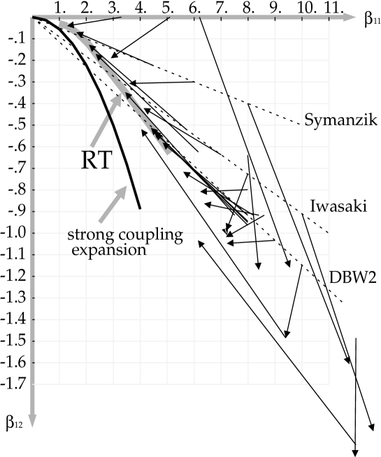
Figure 1: Renormalization group flow for QCD in two coupling space

In Fig.1, the result of the coupling flow is shown. Arrows denote the measured coupling flow. We perform a Monte Carlo simulation with $({{c_{1\times 1}}},{{c_{1\times 2}}})$ (the starting point of an arrow), and then block the lattice. From the blocked links we estimate a blocked action (the end point) through the formula (5) above, by assuming that the blocked action has only two terms, plaquette (${{c_{1\times 1}}}^{\prime}$) and rectangle (${{c_{1\times 2}}}^{\prime}$). It is remarkable that the arrows show a flow of simple structure. They flow into a trajectory. This is a strong evidence that the RT corresponding to this blocking scheme can be seen even in the two-coupling space.

At the strong coupling region, the RT does not look like a linear curve but like a parabolic curve. This is completely consistent with the strong coupling expansion. In the strong coupling regime, $\beta$ is small, and the Boltzmann weight $e^{-\beta S}$ can be expanded as a polynomial in $\beta$. If we include the $1\times 2$ rectangle in the action in addition to the $1\times 1$ plaquette, then the first few loops can easily be evaluated in the regime where $\beta_{1\times 1},\beta_{1\times 2}\ll 1$. In particular, the plaquette and the rectangle give: $\langle W_{11}\rangle\approx\frac{\beta_{1\times 1}}{18}$ , and $\langle W_{12}\rangle\approx(\frac{\beta_{1\times 1}}{18})^{2}+\frac{\beta_{1\times 2}}{18}$. The string tension can then be evaluated at strong coupling as:

$$\sigma a^{2}\approx-\log\frac{\langle W_{12}\rangle}{\langle W_{11}\rangle}=-\log\left(\frac{\beta_{1\times 1}}{18}+\frac{\beta_{1\times 2}}{\beta_{1\times 1}}\right).$$ (6)

Consider now the strong coupling limit $\beta_{1\times 1},\beta_{1\times 2}\rightarrow 0$. The left-hand side should go to $+\infty$, indicating that the lattice spacing $a$ diverges in the strong coupling limit [13].

What is remarkable in the expression for the string tension is that it does not diverge unless $\frac{\beta_{1\times 1}}{18}+\frac{\beta_{1\times 2}}{\beta_{1\times 1}}\rightarrow 0$. In other words, as the renormalized trajectory approaches the high-temperature fixed point (HTFP) ($\beta_{1\times 1}=\beta_{1\times 2}=0$), it must approach the parabola

$$\beta_{1\times 2}=-\frac{1}{18}\beta_{1\times 1}^{2}.$$ (7)

As one goes away from the HTFP along the RT, the lattice spacing shrinks and larger loops must be considered to evaluate the string tension. A straightforward evaluation of the Creutz ratio $\chi_{22}$ already shows that the parabola gets distorted “upwards” as one considers points on the RT further and furtheraway from the HTFP.

On the other hand, in the vicinity of the Ultra-Violet Fixed Point (UVFP), where the lattice spacing is very small, the usual Symanzik improvement (tree-level, tadpole, one-loop or non-perturbative) should be effective at removing ${\cal O}(a^{2})$ cutoff effects. So one expects, as one approaches the UVFP, that the ratio $-\beta_{1\times 2}/\beta_{1\times 1}$ will approach the Symanzik value 0.05. Our MCRG study shows that this ratio is approached from above, as seen also when implementing the Symanzik scheme beyond tree-level. Here we exhibit the smooth connection from the UVFP to the HTFP in the two-coupling plane.

4 Actions in two-coupling space

The analysis in the previous section indicates that along the RT the ratio $-c_{1\times 2}/c_{1\times 1}$ should increase with the lattice spacing, at least until the lattice becomes very coarse. Here we study the rotational symmetry of the heavy quark potential of several approximations to the RT, characterized by a fixed value of $c_{1\times 2}/c_{1\times 1}$.

We parameterize the two-dimensional plane by lines, ${{c_{1\times 1}}}+8{{c_{1\times 2}}}=1$, with ${{c_{1\times 2}}}$ as a parameter; ${{c_{1\times 2}}}=0$ corresponds to the standard Wilson action, ${{c_{1\times 2}}}=-1/12$ to Symanzik’s [14] (tree level with no tadpole improvement), ${{c_{1\times 2}}}=-0.331$ to Iwasaki’s [8]. We include one more steeper line with ${{c_{1\times 2}}}=-1.4088$ which we call DBW2. This line goes through the point obtained after double blocking from a lattice with Wilson action ($\beta=6.3$, $32^{3}\times 64\rightarrow\beta_{1\times 1}\approx 7.986,\beta_{1\times 2}\approx-0.9169$) in 2-dimensional coupling space by the canonical demon method [16].

First let us determine the lattice spacing. We measure the string tension, $\sigma_{phys}a^{2}$ from the heavy quark potential. The heavy quark potential is obtained from Wilson loops $W(R,T)$ calculated from smeared links. The smearing technique proposed in [18] reduces contaminations from excited states to a very large extent.

To determine the heavy quark potential $V(R)$, links are first smeared along the spatial directions; $W(R,T)$ is then computed in terms of the smeared links. The Wilson loops are expected to behave as

$$W(R,T)=C(R)\exp{[-V(R)T]}+\sum C_{i}(R)\exp{[-V_{i}(R)T]}$$ (8)

where $C(R)$ is the overlap function and $V(R)$ is the heavy quark potential, the second term is the contribution from excited states. We obtain $V(R)$ by applying least square fitting to the first term in Eq.(8) as a function of $T$ for each $R$. The fitting range of $T$ is chosen for each $R$ such that the effective mass plots in $T$ become approximately constant neglecting excited states in the fitting. The number of smearing steps is determined so that the overlap function $C(R)$ is closest to one for each $R$.

Next we extract the string tension from $V(R)$. We take the following Ansatz,

$$V(R)=A+\frac{\alpha}{R}+\sigma R$$ (9)

The string tension, $\sigma=\sigma_{phys}a^{2}$, is the coefficient of the linear term in Eq.(9). We fit the heavy quark potential to Eq.(9) in the range where $Ra$ corresponds approximately to physical distances about $0.4fm\sim 1.5fm$. Statistical errors are estimated by the jackknife method with bin size one. We set $\sqrt{\sigma}_{phys}=420MeV$ and fix the scale $a$. Results are summarized in Table 1.

Simulations are performed on a lattice of size $12^{3}\times 24$ . Thermalization is 5000 sweeps, while the interval between Wilson loop measurements is 500 sweeps. The number of configurations used is 100.

action	$\beta$	$\sigma$	$a[\mbox{fm}]$	$\Delta$
Wilson action	5.45	0.463(45)	0.320(16)	0.082(16)
${c_{1\times 1}}=1$	5.55	0.2840(46)	0.2504(20)	0.049(10)
${c_{1\times 2}}=0$	5.65	0.1936(72)	0.2067(38)	0.0254(20)
Symanzik action (tree)	3.70	0.4666(89)	0.3209(31)	0.056(13)
${c_{1\times 1}}=1-8{c_{1\times 2}}$	3.90	0.2634(41)	0.2411(19)	0.0317(53)
${c_{1\times 2}}=-1/12$	4.10	0.1377(48)	0.1743(30)	0.0123(12)
Iwasaki action	1.90	0.6363(72)	0.3748(21)	0.0361(65)
${c_{1\times 2}}=-0.331$	2.00	0.465(13)	0.3204(45)	0.0070(45)
	2.10	0.3496(79)	0.2778(31)	0.0114(27)
	2.20	0.2031(75)	0.2117(39)	0.0057(28)
	2.30	0.1333(63)	0.1715(41)	0.0071(28)
DBW2 action	0.62	0.687(34)	0.3894(96)	0.0147(17)
${c_{1\times 2}}=-1.4088$	0.65	0.512(18)	0.3362(59)	0.0224(50)
	0.70	0.362(13)	0.2827(51)	0.0062(24)
	0.75	0.2489(71)	0.2344(33)	0.0054(16)
	0.80	0.1631(55)	0.1897(12)	0.0078(30)

Table 1: String tensions and the lattice spacing determined from them

If the action lies on the RT, long range quantities behave in the same way as in the continuum. Therefore, even if the lattice is coarse, the rotational symmetry is expected to be recovered. Now we investigate the symmetry breaking in the $({c_{1\times 1}},{c_{1\times 2}})$ plane.

We construct a quantity which measures the amount of rotational symmetry breaking;

$$\Delta^{2}\equiv\sum_{\mbox{off-axis}}\frac{[V(R)-V_{\mbox{on}}(R)]^{2}}{V(R)^{2}\delta V(R)^{2}}\left(\sum_{\mbox{off-axis}}\frac{1}{\delta V(R)^{2}}\right)^{-1}.$$ (10)

where $V_{\mbox{on}}(R)$ is a fit to Eq.(9) determined from on-axis data only. Here “on-axis data” are those on points along a lattice axis. $\delta V(R)$ is the statistical error of $V(R)$. We employ $\Delta$ as a measure of the difference between on-axis and off-axis potential, and therefore a measure of the rotational symmetry breaking. We calculate this quantity with three improved actions at various lattice spacings, i.e., various $\beta$’s.

Results are shown in Table 1 and Fig.2. For small ${c_{1\times 2}}$, like Wilson or tree-level Symanzik actions with no tadpole improvement, $\Delta$ is proportional to $a^{2}$. As $|{c_{1\times 2}}|$ increases, the rotational symmetry is better recovered. To the present accuracy and in the range of couplings studied, the breaking of the rotational symmetry can be already ignored at the level of Iwasaki’s action.

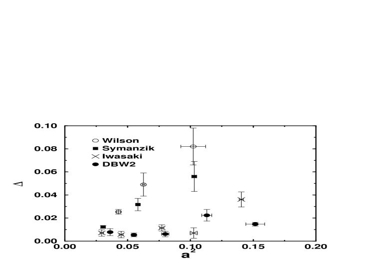
Figure 2: Rotational symmetry breaking

5 Concluding remarks

In this paper, we calculate numerically the RG flow in two-coupling space $({c_{1\times 1}},{c_{1\times 2}})$, as the first step to study the RG flow. Although it is very remarkable that the flow structure can be already observed, the results may have “truncation” errors. After a blocking transformation, the action has in general infinitely many couplings. Therefore end points of the arrows in Fig.1 generally deviate from the two-dimensional plane. To estimate this effect, we calculate the behavior of arrows, whose starting points are near the RT on the two-dimensional plane, in three-dimensional space: $(\beta_{1\times 1},\beta_{1\times 2},\beta_{twist})$, see Fig.3. Deviations from the $(\beta_{1\times 1},\beta_{1\times 2})$ plane are small especially near the RT. This is expected also from the strong coupling expansion: because it takes 3 plaquettes to cover the “twist” loop, its effective coupling will behave like $\beta_{1\times 1}^{3}$ near the HTFP.

Figure 3: RG flow in ($\beta_{1\times 1},\beta_{1\times 2}$) plane, and ($\beta_{1\times 1},\beta_{twist}$) plane.

It is very encouraging that here we have seen a clear flow behavior which strongly indicates the existence of a renormalized trajectory in the vicinity of the 2-coupling plane. We now plan to continue the Monte Carlo RG calculation (i) at higher $\beta$’s, in order to obtain the non-perturbative QCD $\beta$ function, and (ii) in three- or four-coupling space including the chair and twist operators, to estimate truncation effects and evaluate the reliability of the results obtained here.

All simulations have been done on CRAY J90 at Information Processing Center, Hiroshima University, SX-4 at RCNP, Osaka university and on VPP500 at KEK (National Laboratory for High Energy Physics). H.M. would like to thank the Japan Society for the Promotion of Science for Young Scientists for financial support.

References

- [1] K.G. Wilson, in Recent Developments in Gauge theories, ed. G. t’Hooft (Plenum Press, New York, 1980) p.363.
- [2] R. Gupta, “The Renormalization Group and lattice QCD”, From Actions to Answers, ed. T. DeGrand and D. Toussaint, World Scientific 1990; “Scaling, the Renormalization Group and Improved Lattice Actions”, Quantum Fields on the Computer, Ed. M. Creutz, World Scientific, 1992.
- [3] QCDTARO Collaboration, Phys.Rev.Letters,(1993) 71, 3963.
- [4] A. Gonzalez-Arroyo and M. Okawa, Phys.Rev.D 35 (1987) 672; Phys.Rev.B 35 (1987) 2108.
- [5] M. Hasenbusch, K. Pinn and C. Wieczerkowski, Phys. Lett. B338 (1994) 308.
- [6] T. Takaishi, Mod. Phys. Lett. A10 (1995) 503.
- [7] A.Patel and R.Gupta, Phys.Lett. B 183 (1987) 193.
- [8] Y.Iwasaki, University of Tsukuba preprint, UTHEP-118, 1983.
- [9] P. Hasenfratz, F. Niedermayer, Nucl.Phys.B414(1994)785
- [10] QCDTARO Collaboration, Nucl.Phys.B(Proc.Suppl.) 53 (1997) 938.
- [11] R.H. Swendsen, Phys.Rev.Lett. 42 (1979) 859.
- [12] M.Creutz, Phys.Rev.Lett. 50 (1983) 1441 ; M.Hasenbush, K.Pinn, and C.Wieczerkowski, Phys.Lett. B 338 (1994) 308.
- [13] M. Creutz, “Quarks, gluons and lattices”, Cambridge Univ Press, 1985, Chapter 10.
- [14] K.Symanzik, Nucl.Phys.B 226 (1983) 187,205.
- [15] S. Itoh, Y. Iwasaki and T. Yoshie, Phys.Rev.D 33 (1986) 1806.
- [16] T. Takaishi, Phys. Rev. D 54 (1996) 1050.
- [17] I.R. McDonald and K. Singer, Discuss. Faraday, Soc. 43 (1967) 40.; A.M. Ferrenberg and R.H. Swendsen, Phys.Rev.Lett.61 (1988)2635.;63(1989)1195.
- [18] G.S. Bali and K. Schilling, Phys.Rev.D 46(1992) 2636.
- [19] G. Boyd, J. Engels, F. Karsch, E. Laermann, C. Legeland, M. Lütgemeier and B. Petersson, Nucl.Phys.B 469 (1996) 419.
- [20] F. Karsch with B. Beinlich, J. Engels, R. Joswig, E. Laermann, A. Peikert and B. Petersson, Nucl.Phys.B (Proc.Suppl.) 53 (1997) 413.