Non-perturbative determination of anisotropy coefficients
in lattice gauge theories

Abstract

We propose a new non-perturbative method to compute derivatives of gauge coupling constants with respect to anisotropic lattice spacings (anisotropy coefficients), which are required in an evaluation of thermodynamic quantities from numerical simulations on the lattice. Our method is based on a precise measurement of the finite temperature deconfining transition curve in the lattice coupling parameter space extended to anisotropic lattices by applying the spectral density method. We test the method for the cases of $SU(2)$ and $SU(3)$ gauge theories at the deconfining transition point on lattices with the lattice size in the time direction $N_{t}=4$ – 6. In both cases, there is a clear discrepancy between our results and perturbative values. A longstanding problem, when one uses the perturbative anisotropy coefficients, is a non-vanishing pressure gap at the deconfining transition point in the $SU(3)$ gauge theory. Using our non-perturbative anisotropy coefficients, we find that this problem is completely resolved: we obtain $\Delta p/T^{4}=0.001(15)$ and $-0.003(17)$ on $N_{t}=4$ and 6 lattices, respectively.

I Introduction

In order to study the nature of the quark-gluon plasma in heavy ion collisions and in the early Universe, it is important to evaluate the energy density $\epsilon$ and the pressure $p$ near the transition temperature of the deconfining phase transition. These quantities are defined by derivatives of the partition function in terms of the temperature $T$ and the physical volume $V$ of the system

$$\epsilon=-\frac{1}{V}\frac{\partial\ln Z}{\partial T^{-1}},\hskip 14.22636ptp=T\frac{\partial\ln Z}{\partial V}.$$ (1)

The lattice formulation of QCD provides us with a non-perturbative way to compute these quantities by numerical simulations. On a lattice with a size $N_{s}^{3}\times N_{t}$, $V$ and $T$ are given by $V=(N_{s}a_{s})^{3}$ and $T=1/(N_{t}a_{t})$, with $a_{s}$ and $a_{t}$ the lattice spacings in spatial and temporal directions. Because $N_{s}$ and $N_{t}$ are discrete parameters, the partial differentiations in (1) are performed by varying $a_{s}$ and $a_{t}$ independently on anisotropic lattices.

The anisotropy on a lattice is realized by introducing different coupling parameters in temporal and spatial directions. For an $SU(N_{c})$ gauge theory, the standard plaquette action on an anisotropic lattice is given by

$$S=-\beta_{s}\sum_{x,\,i<j\neq 4}P_{ij}(x)-\beta_{t}\sum_{x,\,i\neq 4}P_{i4}(x),$$ (2)

where $P_{\mu\nu}(x)=\frac{1}{N_{c}}{\rm Re\ Tr}\{U_{\mu}(x)U_{\nu}(x+\hat{\mu})U^{\dagger}_{\mu}(x+\hat{\nu})U^{\dagger}_{\nu}(x)\}$ is the plaquette in the $(\mu,\nu)$ plane. With this action, the energy density and pressure are given by [1, 2]

$$\epsilon = -\frac{3N_{t}^{4}T^{4}}{\xi^{3}}\left\{\left(a_{t}\frac{\partial\beta_{s}}{\partial a_{t}}-\xi\frac{\partial\beta_{s}}{\partial\xi}\right)(\langle P_{s}\rangle-\langle P\rangle_{0})+\left(a_{t}\frac{\partial\beta_{t}}{\partial a_{t}}-\xi\frac{\partial\beta_{t}}{\partial\xi}\right)(\langle P_{t}\rangle-\langle P\rangle_{0})\right\},$$ (3)

$$p = \frac{N_{t}^{4}T^{4}}{\xi^{3}}\left\{\xi\frac{\partial\beta_{s}}{\partial\xi}\,(\langle P_{s}\rangle-\langle P\rangle_{0})+\xi\frac{\partial\beta_{t}}{\partial\xi}\,(\langle P_{t}\rangle-\langle P\rangle_{0})\right\},$$ (4)

where $\langle P_{s(t)}\rangle$ is the space(time)-like plaquette expectation value and $\langle P\rangle_{0}$ the plaquette expectation value on a zero-temperature lattice. Here, for later convenience, we have chosen $a_{t}$ and $\xi\equiv a_{s}/a_{t}$ as independent variables to vary the lattice spacings, instead of $a_{s}$ and $\xi$ adopted in [2].

In order to compute $\epsilon$ and $p$ from eqs. (3) and (4) using numerical results from simulations, the values for the derivatives of gauge coupling constants with respect to the anisotropic lattice spacings

$$a_{t}\frac{\partial\beta_{s}}{\partial a_{t}},\hskip 14.22636pta_{t}\frac{\partial\beta_{t}}{\partial a_{t}},\hskip 14.22636pt\frac{\partial\beta_{s}}{\partial\xi},\hskip 14.22636pt\frac{\partial\beta_{t}}{\partial\xi},$$ (5)

which we call the anisotropy coefficients, are required. They can be computed from a requirement that, in the scaling region, the effects of anisotropy in the physical observables can be absorbed by a renormalization of the coupling parameters. Similar to the case of the renormalization group beta-function, the anisotropy coefficients do not depend on the temperature, because the renormalization is independent of the temperature.

The calculation of these anisotropy coefficients in the lowest order perturbation theory is done by Karsch[2]. However, the perturbative coefficients are known to lead to pathological results such as a negative pressure and a non-vanishing pressure gap at the deconfining transition in $SU(3)$ gauge theory. Therefore, non-perturbative values of the anisotropy coefficients are required in order to study the thermodynamic quantities near the phase transition when $N_{t}$ is not sufficiently large.

We are interested in the values of the anisotropy coefficients for isotropic lattices ($\beta_{s}=\beta_{t}\equiv\beta$, i.e. $\xi=1$) where most simulations are performed. In this case, we have $(a_{t}\frac{\partial\beta_{s}}{\partial a_{t}})_{\xi=1}=(a_{t}\frac{\partial\beta_{t}}{\partial a_{t}})_{\xi=1}=a\frac{{\rm d}\beta}{{\rm d}a}=2N_{c}a\frac{{\rm d}g^{-2}}{{\rm d}a}$, where $a\frac{{\rm d}g^{-2}}{{\rm d}a}$ is the beta-function at $\xi=1$, whose non-perturbative values are well studied both in $SU(2)$ and $SU(3)$ gauge theories[3, 4, 5, 6]. Furthermore, a combination of the remaining two anisotropy coefficients is known to be related to the beta-function [2] by

$$\left(\frac{\partial\beta_{s}}{\partial\xi}+\frac{\partial\beta_{t}}{\partial\xi}\right)_{a_{t}:{\rm fixed},\,\xi=1}=\frac{3}{2}\,a\frac{{\rm d}\beta}{{\rm d}a}.$$ (6)

Therefore, only one additional input is required to determine the anisotropy coefficients for isotropic lattices.

A non-perturbative determination of the anisotropy coefficients was attempted in Refs. [7, 8, 9, 10] using a method that we call “the matching method” in the following. One first determines $\xi$ as a function of $\beta_{s}$ and $\beta_{t}$ by matching space-like and time-like Wilson loops on anisotropic lattices, and then numerically determines $\partial\gamma/\partial\xi$ at $\xi=1$, where $\gamma=\sqrt{\beta_{t}/\beta_{s}}$. Interpolation of the Wilson loop data at different sizes or interpolation of $\xi$ at different $\gamma$’s using an Ansatz is required to evaluate $\partial\gamma/\partial\xi$ at $\xi=1$.

Alternatively, we can evaluate a non-perturbative value of pressure directly from the Monte Carlo data by “the integral method” [11]: Assuming homogeneity expected when the spatial lattice size is sufficiently large, we obtain the relation $p=-f$, where $f=-\frac{T}{V}\ln Z$ is the free energy density, which can be evaluated by numerically integrating the plaquette difference $\langle P_{s}\rangle+\langle P_{t}\rangle-2\langle P\rangle_{0}$ in terms of $\beta$ on isotropic lattices. The resulting value of the pressure, in turn, provides us with a non-perturbative estimate of an anisotropy coefficient [4, 5]. In actual numerical simulations, as the value of $p$ in the confining phase and near the deconfining transition point is quite small compared with the magnitude of errors, it is difficult to determine the anisotropy coefficients near the transition point [9].

In this paper, we propose a new method to directly compute the anisotropy coefficients at the deconfining transition point. Our method is described in Sec. II. We test the method in the cases of $SU(2)$ gauge theory in Sec. III. The more realistic case of $SU(3)$ gauge theory is studied in Sec. IV. As an application of our non-perturbative anisotropy coefficients, we study the gaps for $\epsilon$ and $p$ at the $SU(3)$ deconfining transition for $N_{t}=4$ and 6. A summary is given in Sec. V.

II Method

Our method is based on an observation that, in the scaling region, the transition temperature $T_{c}=1/\{N_{t}a_{t}(\beta_{s},\beta_{t})\}$ must be independent of the anisotropy of the lattice. Therefore, when we change the coupling constants along the transition curve in the $(\beta_{s},\beta_{t})$ plane like $(\beta_{s},\beta_{t})\rightarrow(\beta_{s}+{\rm d}\beta_{s},\beta_{t}+{\rm d}\beta_{t})$ on a lattice with fixed $N_{t}$, the lattice spacing in the time direction $a_{t}$ does not change:

$${\rm d}a_{t}=\frac{\partial a_{t}}{\partial\beta_{s}}\,{\rm d}\beta_{s}+\frac{\partial a_{t}}{\partial\beta_{t}}\,{\rm d}\beta_{t}=0.$$ (7)

We denote the slope of the transition curve at $\xi=1$ by $r_{t}$;

$$r_{t}=\frac{{\rm d}\beta_{s}}{{\rm d}\beta_{t}}=-\left(\frac{\partial a_{t}}{\partial\beta_{t}}\right)_{\xi=1}\left/\left(\frac{\partial a_{t}}{\partial\beta_{s}}\right)_{\xi=1}\right.=\left(\frac{\partial\beta_{s}}{\partial\xi}\right)_{\xi=1}\left/\left(\frac{\partial\beta_{t}}{\partial\xi}\right)_{\xi=1}\right.,$$ (8)

where we used an identity

$$\left(\begin{array}[]{cc}\frac{\partial\beta_{s}}{\partial a_{t}}&\frac{\partial\beta_{t}}{\partial a_{t}}\\ \frac{\partial\beta_{s}}{\partial\xi}&\frac{\partial\beta_{t}}{\partial\xi}\end{array}\right)=\frac{1}{\frac{\partial\xi}{\partial\beta_{t}}\frac{\partial a_{t}}{\partial\beta_{s}}-\frac{\partial\xi}{\partial\beta_{s}}\frac{\partial a_{t}}{\partial\beta_{t}}}\left(\begin{array}[]{cc}\frac{\partial\xi}{\partial\beta_{t}}&-\frac{\partial\xi}{\partial\beta_{s}}\\ -\frac{\partial a_{t}}{\partial\beta_{t}}&\frac{\partial a_{t}}{\partial\beta_{s}}\end{array}\right).$$ (13)

Hence, the derivatives of $\beta_{s}$ and $\beta_{t}$ in terms of $\xi$ are expressed as

$$\left(\frac{\partial\beta_{s}}{\partial\xi}\right)_{\xi=1} = \frac{3r_{t}}{2(1+r_{t})}\,a\frac{{\rm d}\beta}{{\rm d}a},$$ (14)

$$\left(\frac{\partial\beta_{t}}{\partial\xi}\right)_{\xi=1} = \frac{3}{2(1+r_{t})}\,a\frac{{\rm d}\beta}{{\rm d}a}.$$ (15)

Introducing the conventional notation $\gamma=\sqrt{\beta_{t}/\beta_{s}}$ and $\beta=\sqrt{\beta_{s}\beta_{t}}$, we obtain

$$\left(\frac{\partial\gamma}{\partial\xi}\right)_{a_{t}:{\rm fixed},\,\xi=1}=\left(\frac{\partial\gamma}{\partial\xi}\right)_{a_{s}:{\rm fixed},\,\xi=1}=\frac{3}{4\beta}\,\frac{1-r_{t}}{1+r_{t}}\,a\frac{{\rm d}\beta}{{\rm d}a}.$$ (16)

Finally, the customarily used forms for the anisotropy coefficients (Karsch coefficients) [2] are given by

$$c_{s} = \left(\frac{\partial g_{s}^{-2}}{\partial\xi}\right)_{a_{s}:{\rm fixed},\,\xi=1}=\frac{1}{2N_{c}}\left\{\beta+\frac{r_{t}-2}{2(1+r_{t})}\,a\frac{{\rm d}\beta}{{\rm d}a}\right\},$$ (17)

$$c_{t} = \left(\frac{\partial g_{t}^{-2}}{\partial\xi}\right)_{a_{s}:{\rm fixed},\,\xi=1}=\frac{1}{2N_{c}}\left\{-\beta+\frac{1-2r_{t}}{2(1+r_{t})}\,a\frac{{\rm d}\beta}{{\rm d}a}\right\},$$ (18)

where $\beta_{s}=2N_{c}g_{s}^{-2}\xi^{-1}$ and $\beta_{t}=2N_{c}g_{t}^{-2}\xi$. Therefore, when the value for the beta-function is available, we can determine these anisotropy coefficients by measuring $r_{t}$ from the finite temperature transition curve in the $(\beta_{s},\beta_{t})$ plane.

In order to determine the transition curve in the coupling parameter space, we compute the rotated Polyakov loop

$$L=z\,\frac{1}{N_{s}^{3}}\sum_{\vec{x}}\frac{1}{N_{c}}{\rm Tr}\prod_{t=1}^{N_{t}}U_{4}(\vec{x},t)$$ (19)

as a function of $(\beta_{s},\beta_{t})$, where $z$ is a $Z(N_{c})$ phase factor ($z^{N_{c}}=1$) such that $\arg(L)\in(-\pi/N_{c},\pi/N_{c}]$. We define the transition point as the peak position of the susceptibility $\chi=N_{s}^{3}(\langle L^{2}\rangle-\langle L\rangle^{2})$ in $\beta$ for each fixed $\gamma$.

We compute the coupling parameter dependence of $\chi$ in the $(\beta_{s},\beta_{t})$ plane by applying the spectral density method [13] extended to anisotropic lattices. This enables us to compute the anisotropy coefficients directly from simulations at $\xi\approx 1$ without introducing an interpolation Ansatz. Another good feature of the spectral density method is that the method works well even with data obtained only on isotropic lattices. Therefore, we can use data from previous high statistic simulations performed on isotropic lattices, when the time histories of the Polyakov loop and space-like and time-like plaquettes are available near the transition point.

Fitting the transition curve with a polynomial

$$\beta_{c}(\gamma)=\sum_{n=0}^{n_{\rm max}}f_{n}\,(\gamma-1)^{n},$$ (20)

with $f_{n}$ the fitting parameters, the slope $r_{t}$ is given by

$$r_{t}=\left(\frac{{\rm d}(\beta_{c}/\gamma)}{{\rm d}(\beta_{c}\gamma)}\right)_{\xi=1}=\frac{({\rm d}\beta_{c}/{\rm d}\gamma)_{\xi=1}-\beta_{c}}{({\rm d}\beta_{c}/{\rm d}\gamma)_{\xi=1}+\beta_{c}},$$ (21)

where $({\rm d}\beta_{c}/{\rm d}\gamma)_{\xi=1}=f_{1}.$ The range of $\beta$ and $\gamma$ in which the spectral density method is reliable is estimated by the condition that the statistical error for the reweighting factor (which is $\langle e^{-\Delta S}\rangle$ when the number of simulation points is one) is less than 0.5%. We confirm that the results are completely stable under a variation of $n_{\rm max}$ when we restrict ourselves to the range discussed above. Choosing a range of $\gamma$ around 1 in such a way that the transition curve is almost straight, we use $n_{\rm max}=3$ for the final results.

III Results for $SU(2)$

We first test the method for the case of $SU(2)$ gauge theory at the transition point $\beta_{c}$ for $N_{t}=4$ and 5. Although the method should work well with data only from isotropic lattices, in order to confirm it, we perform Monte Carlo simulations also on several anisotropic lattices for $SU(2)$. On a $16^{3}\times 4$ lattice, we perform simulations at $(\beta_{s},\beta_{t})=(2.300,2.300)$, (2.302, 2.302), (2.296, 2.306), and (2.307, 2.298). On a $20^{3}\times 5$ lattice, we simulate at $(\beta_{s},\beta_{t})=(2.373,2.373)$, (2.375,2.375), (2.380,2.370) and (2.368,2.378). At each $(\beta_{s},\beta_{t})$ on the $N_{t}=4$ (5) lattice, we accumulate 500,000 (1,250,000) configurations, each separated by 10 heat-bath sweeps, after thermalization. The statistical errors are estimated using the jackknife method with the bin size of 1000 configurations. We confirm that the errors are stable under a wide variation of the bin size around this value.

Computing the susceptibility in the $(\beta_{s},\beta_{t})$ plane using data at each simulation point, we check that the results agree well with each other, i.e. the results for the susceptibility from isotropic lattices coincide with the results from anisotropic lattices. For the rest of this section, we combine the results for all four $(\beta_{s},\beta_{t})$ combinations to compute the susceptibility with the spectral density method. In Fig.1, we plot the susceptibility for $N_{t}=4$ at $\gamma=0.995$, 1.000, and 1.005. The results for the peak position $\beta_{c}$ of the susceptibility computed at various values of $\gamma$ are summarized in Fig. 2 for $N_{t}=4$ and 5.

Fitting the results for the transition curve, we obtain the values for $\beta_{c}$ and $r_{t}$ at $\xi=1$, as summarized in Table I. Combining the values of $r_{t}$ with a result of the $SU(2)$ beta-function[4] at $\beta_{c}(\xi\!=\!1)$, we obtain the anisotropy coefficients (16) and (18). The results are summarized in Table II. Because no errors for the beta-function are given in [4], we disregard their contribution to the errors of the anisotropy coefficients.

In Fig. 3, we compare our results for the Karsch coefficients with the results of the perturbation theory (dot-dashed curves) [2] and the integral method (dotted curves) [4]. We find significant discrepancies between our results and the results of the perturbation theory. On the other hand, our results are consistent with the results from the integral method.

IV Results for $SU(3)$

Let us now study the more realistic case of the $SU(3)$ gauge theory. We analyze the high statistic data for the $SU(3)$ gauge theory obtained by the QCDPAX Collaboration [14]. Simulations were performed at the deconfining transition point for $N_{t}=4$ and 6. For $N_{t}=4$, the lattice sizes are $24^{2}\times 36\times 4$ and $12^{3}\times 24\times 4$, with $712\,000$ and $910\,000$ pseudo heat-bath iterations, respectively. For $N_{t}=6$, data on $36^{2}\times 48\times 6$, $24^{3}\times 6$, and $20^{3}\times 6$ lattices with $1\,112\,000$, $480\,000$, and $376\,000$ iterations are available. The Polyakov loop and the plaquettes are measured every iteration. Details of the simulation parameters are given in [14]. For the bin size in the jack-knife analysis, we adopt the same values as in [14].

A Anisotropy coefficients

The results for the susceptibility on the largest spatial lattices are given in Figs. 4 and 5. Because the transition is of first order for $SU(3)$, the peak of the susceptibility is quite clear when the spatial lattice size is large enough, as shown in Figs. 4 and 5. (Note the difference in the vertical scales between Figs. 1 and 4.)

Our results for the slope $r_{t}$ are summarized in Table III. Except for the case of the $24^{3}\times 6$ lattice where the simulation point is slightly off the transition point, the errors become larger with decreasing spatial volume, because the peak of the susceptibility becomes less clear on small lattices. From Table III, we find that the slopes at $N_{t}=4$ with different spatial lattice volumes completely agree with each other. As shown in Figs. 4 and 5, the peak of the susceptibility for $N_{t}=6$ is less sharp compared with that for $N_{t}=4$ with the same relative spatial volume $(N_{s}/N_{t})^{3}$ due to the fact that the transition is weaker for $N_{t}=6$ [14]. Therefore, with comparable statistics, $r_{t}$ has a larger statistical error for $N_{t}=6$. Unlike in the case of $N_{t}=4$, the central values for the slope for $N_{t}=6$ given in Table III vary with the spatial volume by about one standard deviation. However, because the volume dependence is not uniform, we consider that it is caused by statistical fluctuations. We use the values obtained on the largest spatial lattices for our final results.

Our results for the anisotropy coefficients are summarized in Table IV. For our final results, we adopt the beta-function computed from a recent string tension data by the SCRI group [6]. See a subsection below for a discussion about the influence on the results from the choice of the beta-function.

B Pressure gap and latent heat

As an application of our non-perturbative anisotropy coefficients, we reanalyze the thermodynamic quantities $\epsilon$ and $p$ at the deconfining transition point using the plaquette data by the QCDPAX Collaboration [14]. In terms of the slope $r_{t}$ and the beta-function, the conventional combinations $\epsilon-3p$ and $\epsilon+p$ are given by

$$(\epsilon-3p)/T^{4} = -3N_{t}^{4}\,a\frac{{\rm d}\beta}{{\rm d}a}\,\{\langle P_{s}\rangle+\langle P_{t}\rangle\ -2\langle P\rangle_{0}\},$$ (22)

$$(\epsilon+p)/T^{4} = 3N_{t}^{4}\,a\frac{{\rm d}\beta}{{\rm d}a}\,\frac{r_{t}-1}{r_{t}+1}\,\{\langle P_{s}\rangle-\langle P_{t}\rangle\}.$$ (23)

At a first order transition point, we have a finite gap for energy density, the latent heat, but expect no gap for pressure. It is known that the perturbative anisotropy coefficients have a difficulty which leads to a non-vanishing pressure gap at the deconfining transition point: $\Delta p/T^{4}=-0.32(3)$ and $-0.14(2)$ at $N_{t}=4$ and 6 [14].

New values for the gaps in $\epsilon$ and $p$ using our non-perturbative anisotropy coefficients are summarized in Table V. For the pressure gap, we obtain

$$\Delta p/T^{4}=\left\{\begin{array}[]{rc}0.001(15)&\;\mbox{for $N_{t}=4$,}\\ -0.003(17)&\;\mbox{for $N_{t}=6$.}\end{array}\right.$$ (26)

We find that the problem of non-zero pressure gap is completely resolved with our non-perturbative anisotropy coefficients.

C Choice of the beta-function

In Table IV, we study the influence of the choice of the beta-function on the anisotropy coefficients. We compare (i) the beta-function computed from a recent string tension data by the SCRI group [6], (ii) that from a MCRG study by the QCDTARO Collaboration [3], and (iii) that from a study of $\beta_{c}(N_{t})$ by the Bielefeld group [5]. The SCRI beta-function is computed using a fit of the string tension for $5.6\leq\beta\leq 6.5$. We note that the QCDTARO beta-function is based on a fit of mean-field improved gauge coupling constant using the results of plaquette at $\beta>5.8$; i.e. $\beta_{c}(N_{t}\!=\!4)\approx 5.69$ is slightly off the range of validity [3, 15]. Also the beta-function by the Bielefeld group seems to be problematic around $\beta_{c}(N_{t}\!=\!4)$, because it is largely affected by the data of $\beta_{c}(N_{t}\!=\!3)$ where we cannot expect universal scaling. Accordingly, the beta-function of the Bielefeld group shows a systematic deviation from the data of a MCRG study at $\beta$ $<$$\sim$ 6 [5].

These beta-functions are plotted in Fig. 6. At $\beta_{c}(N_{t}\!=\!6)$, different beta-functions coincide with each other within 5%, while, at $\beta_{c}(N_{t}\!=\!4)$, they vary by about 20%. Because only the SCRI beta-function is reliable at $\beta_{c}(N_{t}\!=\!4)$ as discussed in the previous paragraph, we adopt the SCRI beta-function for our final results.

In order to compare the anisotropy coefficients from different references, however, it is important to check the effect of the beta-function on the results. From Table IV, we see that the results for the anisotropy coefficients using different beta-functions agree well with each other at $N_{t}=6$. At $N_{t}=4$, however, the anisotropy coefficients depend very much on the choice of the beta-function. Accordingly, we find that the results for the latent heat are consistent with each other at $N_{t}=6$: $\Delta\epsilon/T^{4}=1.569(40)$, 1.539(39), and 1.515(38) with SCRI, QCDTARO, and Bielefeld beta-functions, respectively. At $N_{t}=4$, we find a sizable dependence on the choice of the beta-function: $\Delta\epsilon/T^{4}=2.074(34)$, 1.877(30), and 2.265(37) using SCRI, QCDTARO, and Bielefeld beta-functions. For the pressure gap, on the other hand, because the beta-function appears only as a common overall factor in (22) and (23), the conclusion that $\Delta p$ vanishes with our anisotropy coefficients does not depend on the choice of the beta-function.

D Comparison with other methods

In Fig. 7, we summarize our results for the Karsch coefficients together with previous values; the perturbative results [2], results from the integral method [5], and those from the matching of Wilson loops on anisotropic lattices [9, 10]. No errors are published for the results from the integral method. We find that all non-perturbative methods give values which deviate from the results in the perturbation theory.

Comparing the results from different non-perturbative methods, we find that, although the deviations from the perturbation theory are roughly consistent with each other, the central values are different by more than three standard deviations, when we take the published errors.

We think that one origin of the variation among different methods at $\beta_{c}(N_{t}\!=\!4)$ is the beta-function. Note that the results from Refs. [9] (matching method) and [5] (integral method) are computed using the beta-function of the Bielefeld group, while our results and the results from Ref. [10] (matching method) are using the SCRI beta-function. From Table IV, we note that, if we adopt the beta-function of the Bielefeld group, our results are consistent with those of Ref. [9] at $\beta_{c}(N_{t}\!=\!4)$.

At $\beta_{c}(N_{t}\!=\!6)$, on the other hand, the difference in the results is not due to the beta-function, because the systematic error due to the choice of the beta-function is small as discussed in the previous subsection. In order to see this, we study $\partial\gamma/\partial\xi$, which can be computed without using the beta-function in the matching method. The values of $\partial\gamma/\partial\xi$ obtained in Ref. [10] are reported to be consistent with those from the integral method [5], but are different to another result from the matching method [9]. Performing a quadratic interpolation in $\beta$, we find $\partial\gamma/\partial\xi\simeq 0.64(1)$ [10], $0.66(2)$ [5], and $0.74(2)$ [9] at $\beta_{c}(N_{t}\!=\!6)$. Our result $0.707(10)$ given in Table IV is around the center of these values. A careful study of systematic errors in each method is required to understand the variation between different methods.

V Conclusions

We have computed the anisotropy coefficients for the $SU(2)$ and $SU(3)$ gauge theories by measuring the transition curve of the deconfining transition in the $(\beta_{s},\beta_{t})$ plane. One of the essential ingredients of our approach is the application of the spectral density method, that enables us to determine the anisotropy coefficients directly from simulations at $\xi\approx 1$. We note that the spectral density method is useful to avoid interpolation Ansätze also in the matching method.

Our non-perturbative results for the anisotropy coefficients are summarized in Tables II and IV. Our results shown in Fig. 7 suggest that the Karsch coefficients converge to the perturbative values slightly faster than that suggested by the central values from Refs. [5] and [10]. Applying the results for $SU(3)$, we reanalyzed the thermodynamic quantities at the deconfining transition point on $N_{t}=4$ and 6 lattices. We obtain vanishing pressure gaps with our non-perturbative anisotropy coefficients, thereby solving a longstanding problem of non-zero pressure gap with the perturbative coefficients.

We are grateful to O. Miyamura, A. Nakamura and H. Matsufuru for useful discussions and sending us the data for the QCDTARO beta-function. We also thank A. Ukawa, T. Yoshié, Y. Aoki, T. Kaneko, R. Burkhalter and H.P. Shanahan for helpful suggestions and comments. This work is in part supported by the Grants-in-Aid of Ministry of Education, Science and Culture (Nos. 08NP0101 and 09304029). SE is supported by the Japan Society for the Promotion of Science.

TABLE I.: Results for $\beta_{c}$ and the slopes at $\xi=1$ in the $SU(2)$ gauge theory. The column “$\gamma$-range” is for the range of $\gamma$ used in the fit for the slope $d\beta_{c}/d\gamma$.

lattice	$\beta_{c}$	$\gamma$-range	$d\beta_{c}/d\gamma$	$r_{t}$
$16^{3}\times 4$	2.30177(9)	0.995 – 1.005	$-$0.370(12)	$-$1.384(14)
$20^{3}\times 5$	2.37430(8)	0.995 – 1.005	$-$0.312(15)	$-$1.303(17)

TABLE II.: $SU(2)$ anisotropy coefficients at $\xi=1$ using the beta-function $a{\rm d}g^{-2}/{\rm d}a$ obtained by the Bielefeld group [4].

lattice	$\partial\gamma/\partial\xi$	$c_{s}$	$c_{t}$	$a{\rm d}g^{-2}/{\rm d}a$
$16^{3}\times 4$	0.683(21)	0.203(12)	$-$0.161(12)	$-$0.08439
$20^{3}\times 5$	0.725(35)	0.182(21)	$-$0.144(21)	$-$0.07544

TABLE III.: The same as Table I for $SU(3)$ using the data by the QCDPAX Collaboration [14].

lattice	$\beta_{c}$	$\gamma$-range	$d\beta_{c}/d\gamma$	$r_{t}$
$24^{2}\times 36\times 4$	5.69245(23)	0.9975 – 1.0025	$-$0.5193(23)	$-$1.2008(10)
$12^{2}\times 24\times 4$	5.69149(42)	0.995 – 1.005	$-$0.5183(52)	$-$1.2004(22)
$36^{2}\times 48\times 6$	5.89379(34)	0.999 – 1.001	$-$0.5844(83)	$-$1.2201(35)
$24^{3}\times 6$	5.89292(87)	0.999 – 1.001	$-$0.542(33)	$-$1.202(14)
$20^{3}\times 6$	5.8924(14)	0.9975 – 1.0025	$-$0.622(34)	$-$1.236(14)

TABLE IV.: $SU(3)$ anisotropy coefficients at $\xi=1$, using the values for the beta-function $a{\rm d}g^{-2}/{\rm d}a$ by the SCRI group[6], the QCDTARO Collaboration[3], and the Bielefeld group[5]. For our final results, we take the values obtained on the largest spatial lattices using the SCRI beta-function. Because the errors for the beta-function are not given in the papers, we disregard their contribution to the errors of the anisotropy coefficients in this table. See text for details.

lattice	$\partial\gamma/\partial\xi$	$c_{s}$	$c_{t}$	$a{\rm d}g^{-2}/{\rm d}a$
$24^{2}\times 36\times 4$	0.6159(27)	0.3822(26)	$-$0.3466(26)	$-$0.07108     SCRI
	0.5575(25)	0.4359(23)	$-$0.4037(23)	$-$0.06434     QCDTARO
	0.6728(30)	0.3299(28)	$-$0.2910(28)	$-$0.07764     Bielefeld
$12^{2}\times 24\times 4$	0.6161(62)	0.3819(59)	$-$0.3464(59)	$-$0.07097     SCRI
	0.5573(56)	0.4360(53)	$-$0.4039(53)	$-$0.06418     QCDTARO
	0.6738(68)	0.3288(64)	$-$0.2900(64)	$-$0.07761     Bielefeld
$36^{2}\times 48\times 6$	0.7068(100)	0.3109(98)	$-$0.2650(98)	$-$0.09179     SCRI
	0.6936(98)	0.3235(96)	$-$0.2784(96)	$-$0.09008     QCDTARO
	0.6826(96)	0.3340(95)	$-$0.2897(95)	$-$0.08864     Bielefeld
$24^{3}\times 6$	0.762(47)	0.257(46)	$-$0.211(46)	$-$0.09172     SCRI
	0.747(46)	0.271(45)	$-$0.226(45)	$-$0.08999     QCDTARO
	0.736(45)	0.282(45)	$-$0.237(45)	$-$0.08857     Bielefeld
$20^{3}\times 6$	0.663(36)	0.354(35)	$-$0.308(35)	$-$0.09167     SCRI
	0.651(35)	0.366(35)	$-$0.321(35)	$-$0.08994     QCDTARO
	0.640(35)	0.375(34)	$-$0.331(34)	$-$0.08853     Bielefeld

TABLE V.: Gaps for thermodynamic quantities in the $SU(3)$ gauge theory at the deconfining transition point using our non-perturbative anisotropy coefficients. Plaquette data are taken from Ref. [14]. The low temperature hadronic phase (had) and the high temperature quark-gluon-plasma phase (QGP) are separated as described in [14]. We reanalyze $(\epsilon-3p)/T^{4}$ also, using the SCRI beta-function.

lattice	$24^{2}\times 36\times 4$	$36^{2}\times 48\times 6$
$\beta$	5.6925	5.8936
$\Delta(\epsilon+p)/T^{4}$	2.075(42)	1.565(51)
$\Delta(\epsilon-3p)/T^{4}$	2.072(43)	1.578(42)
$\Delta\epsilon/T^{4}$	2.074(34)	1.569(40)
$\Delta p/T^{4}$	0.001(15)	$-$0.003(17)

FIG. 1.: Polyakov loop susceptibility in the $SU(2)$ gauge theory on a $16^{3}\times 4$ lattice at $\gamma=0.995$, 1.0 and 1.005. Errors are estimated by a jackknife method.

(a)

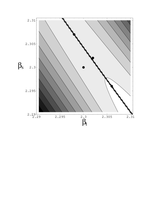
(b)

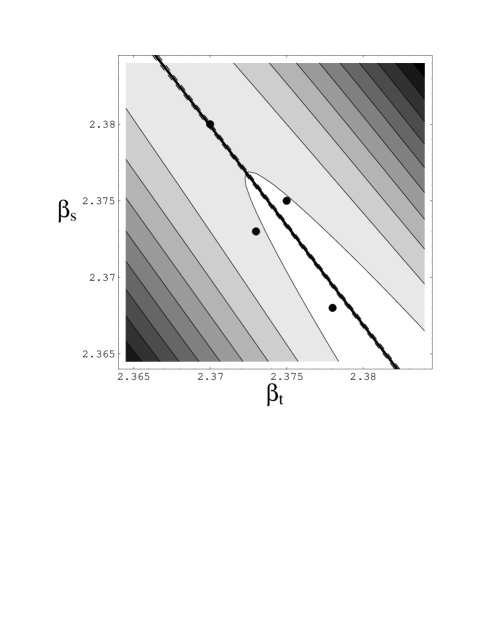
FIG. 2.: Polyakov loop susceptibility in the $SU(2)$ gauge theory as a function of $(\beta_{s},\beta_{t})$ obtained on (a) $16^{3}\times 4$ and (b) $20^{3}\times 5$ lattices. Simulation points are shown by filled circles. The bold lines represent the peak position of the susceptibility and the dashed lines their errors. The magnitude of the susceptibility is shown by tone for the range (a) $8.2<\chi<10.4$ and (b) $9.0<\chi<11.2$, respectively, where different tone corresponds to a difference $\Delta\chi=0.2$.

FIG. 3.: Anisotropy coefficients $c_{s}$ and $c_{t}$ for the $SU(2)$ gauge theory. Our non-perturbative results are given by filled circles. The dot-dashed curves are the results of the perturbation theory [2]. The dotted curves are the results from the integral method [4]. No errors are published for these curves.

(a)

(b)

FIG. 4.: Polyakov loop susceptibility in the $SU(3)$ gauge theory obtained (a) on the $24^{2}\times 36\times 4$ lattice at $\gamma=0.9975$, 1.0 and 1.0025, and (b) on the $36^{2}\times 48\times 6$ lattice at $\gamma=0.999$, 1.0 and 1.001.

(a)

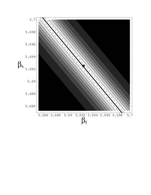
(b)

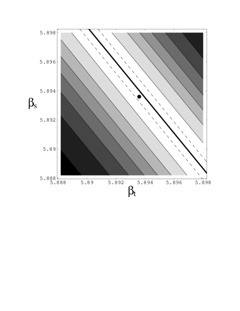
FIG. 5.: The same as Fig. 2 for the $SU(3)$ gauge theory on (a) $24^{3}\times 36\times 4$ and (b) $36^{2}\times 48\times 6$ lattices. The range of $\chi$ plotted and the width $\Delta\chi$ for a tone are (a) 0.0 – 45.0, 5.0 and (b) 2.5 – 22.5, 2.5, respectively.

FIG. 6.: Non-perturbative beta-functions in the $SU(3)$ gauge theory.

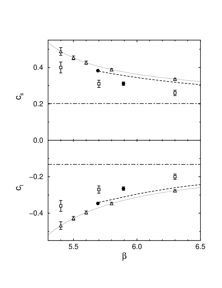
FIG. 7.: Anisotropy coefficients in the $SU(3)$ gauge theory. Our non-perturbative results are given by filled circles. The dot-dashed curves are the results of the perturbation theory [2]. The open squares are those from a matching of Wilson loops [9]. Open triangles and thin lines are the results of a matching method [10] combined with the SCRI beta-function [6]. The dotted curves are the results from the integral method [5]. No errors are published for the results from the integral method.

REFERENCES

- [1] J. Engels, F. Karsch, H. Satz and I. Montvay, Nucl. Phys. B205 (1982) 545.
- [2] F. Karsch, Nucl. Phys. B205 (1982) 285.
- [3] K. Akemi et al., Phys. Rev. Lett. 71 (1993) 3063.
- [4] J. Engels, F. Karsch and K. Redlich, Nucl. Phys. B435 (1995) 295.
- [5] G. Boyd et al., Nucl. Phys. B469 (1996) 419.
- [6] R.G. Edwards, U.M. Heller and T.R. Klassen, hep-lat/9711003.
- [7] G. Burgers, F. Karsch, A. Nakamura and I.O. Stamatescu, Nucl. Phys. B304 (1988) 587.
- [8] M. Fujisaki et al., Nucl. Phys. B(Proc. Suppl.)53 (1997) 426.
- [9] J. Engels, F. Karsch and T. Scheideler, Nucl. Phys. B(Proc. Suppl.)63 (1998) 427.
- [10] T.R. Klassen, hep-lat/9803010.
- [11] J. Engels et al., Phys. Lett. B252 (1990) 625.
- [12] I. Montvay and E. Pietarinen, Phys. Lett. B110 (1982) 148.
- [13] A.M. Ferrenberg and R.H. Swendsen, Phys. Rev. Lett. 61 (1988) 2635; Phys. Rev. Lett. 63 (1989) 1195.
- [14] Y. Iwasaki, K. Kanaya, T. Yoshié, T. Hoshino, T. Shirakawa, Y. Oyanagi, S. Ichii, and T. Kawai, Phys. Rev. D46 (1992) 4657.
- [15] O. Miyamura and A. Nakamura, private communication.