Instantons and Monopoles in the Nonperturbative QCD

1 Dual Superconductor Picture for Confinement in QCD

Quantum Chromodynamics (QCD) shows the asymptotic freedom due to its nonabelian nature, and the perturbative calculation is workable in the ultraviolet region as $\mathchar 28950\relax\gg$ 1GeV. On the other hand, in the infrared region as $\mathchar 28950\relax\mathop{{}^{<}}_{\!\!\!\!\!\sim}$ 1GeV, QCD exhibits nonperturbative phenomena like color confinement and dynamical chiral-symmetry breaking (D$\mathchar 28959\relax$SB) due to the strong-coupling nature. Up to now, there is no systematic promising method for the study of the nonperturbative QCD (NP-QCD) except for the lattice QCD calculation with the Monte Carlo method.

The lattice QCD simulation can be regarded as a numerical experiment based on the rigid field-theoretical framework, and provides a powerful technique for the analyses of the NP-QCD vacuum and hadrons. Owing to the great progress of the computer power in these days, the lattice QCD becomes useful not only for “reproductions of hadron properties” but also for “new predictions” like glueball properties and the QCD phase transition. The “physical understanding” for NP-QCD is also one of the most important subjects in the lattice QCD, because the aim of theoretical physics is never to reproduce numbers but to find the “physical mechanism” hidden in phenomena ! In this paper, we study the confinement physics in QCD using both the lattice QCD and the theoretical formalism.

In 1974, Nambu proposed an interesting idea that quark confinement would be physically interpreted using the dual version of the superconductivity.¹ In the ordinary superconductor, Cooper-pair condensation leads to the Meissner effect, and the magnetic flux is excluded or squeezed like a quasi-one-dimensional tube as the Abrikosov vortex, where the magnetic flux is quantized topologically. On the other hand, from the Regge trajectory of hadrons and the lattice QCD results, the confinement force between the color-electric charge is characterized by the universal physical quantity of the string tension, and is brought by one-dimensional squeezing of the color-electric flux in the QCD vacuum. Hence, the QCD vacuum can be regarded as the dual version of the superconductor based on above similarities on the low-dimensionalization of the quantized flux between charges.

In the dual-superconductor picture for the QCD vacuum, the squeezing of the color-electric flux between quarks is realized by the dual Meissner effect, as the result of condensation of color-magnetic monopoles, which is the dual version of the electric charge as the Cooper pair. However, there are two large gaps between QCD and the dual-superconductor picture.²

(1) This picture is based on the abelian gauge theory subject to the Maxwell-type equations, where electro-magnetic duality is manifest, which QCD is a nonabelian gauge theory.

(2) The dual-superconductor scenario requires condensation of (color-)magnetic monopoles as the key concept, while QCD does not have such a monopole as the elementary degrees of freedom.

As the connection between QCD and the dual-superconductor scenario, ’t Hooft proposed the concept of the abelian gauge fixing,³ the partial gauge fixing which only remains abelian gauge degrees of freedom in QCD. By definition, the abelian gauge fixing reduces QCD into an abelian gauge theory, where the off-diagonal element of the gluon field behaves as a charged matter field similar to $W^{\pm}_{\mathchar 28950\relax}$ in the Standard Model and provides a color-electric current in terms of the residual abelian gauge symmetry. As a remarkable fact in the abelian gauge, color-magnetic monopoles appear as topological objects corresponding to the nontrivial homotopy group $\mathchar 28933\relax_{2}({\rm SU(N_{c})/U(1)}^{\rm N_{c}-1})$ $={\bf Z}^{\rm N_{c}-1}_{\infty}$ in a similar manner to the GUT monopole.^3-6 In general, the monopole appears as a topological defect or a singularity in a constrained abelian gauge manifold embedded in the compact (and at most semi-simple) nonabelian gauge manifold.

Here, let us consider appearance of monopoles in terms of the gauge connection. In the general system including the singularities such as the Dirac string, the field strength is defined as

$$G_{\mathchar 28950\relax\mathchar 28951\relax}\equiv\frac{1}{ie}([\hat{D}_{\mathchar 28950\relax},\hat{D}_{\mathchar 28951\relax}]-[\hat{\partial}_{\mathchar 28950\relax},\hat{\partial}_{\mathchar 28951\relax}]),$$ (1.1)

which takes a form of the difference between the covariant derivative operator $\hat{D}_{\mathchar 28950\relax}\equiv\hat{\partial}_{\mathchar 28950\relax}+ieA_{\mathchar 28950\relax}(x)$ and the derivative operator $\hat{\partial}$ satisfying $[\hat{\partial}_{\mathchar 28950\relax},f(x)]=\partial_{\mathchar 28950\relax}f(x)$. By the general gauge transformation with the gauge function $\mathchar 28938\relax$, the field strength $G_{\mathchar 28950\relax\mathchar 28951\relax}$ is transformed as

$$G_{\mathchar 28950\relax\mathchar 28951\relax}\equiv\frac{1}{ie}\rightarrow{G^{\prime}}_{\mathchar 28950\relax\mathchar 28951\relax} \equiv \mathchar 28938\relax G_{\mathchar 28950\relax\mathchar 28951\relax}\mathchar 28938\relax^{\dagger}=\frac{1}{ie}([\hat{D^{\prime}}_{\mathchar 28950\relax},\hat{D^{\prime}}_{\mathchar 28951\relax}]-\mathchar 28938\relax[\hat{\partial}_{\mathchar 28950\relax},\hat{\partial}_{\mathchar 28951\relax}]\mathchar 28938\relax^{\dagger})$$ (1.2)

$$= \partial_{\mathchar 28950\relax}{A^{\prime}}_{\mathchar 28951\relax}-\partial_{\mathchar 28951\relax}{A^{\prime}}_{\mathchar 28950\relax}+ie[{A^{\prime}}_{\mathchar 28950\relax},{A^{\prime}}_{\mathchar 28951\relax}]+\frac{i}{e}\mathchar 28938\relax[\partial_{\mathchar 28950\relax},\partial_{\mathchar 28951\relax}]\mathchar 28938\relax^{\dagger}.$$ (1.3)

The last term remains only for the singular gauge transformation, and can provide the Dirac string in the abelian gauge sector. For a singular ${\rm SU}(N_{c})$ gauge function, the last term leads to breaking of the abelian Bianchi identity and monopoles in the abelian gauge.

Thus, by the abelian gauge fixing, QCD is reduced into an abelian gauge theory including both the electric current $j_{\mathchar 28950\relax}$ and the magnetic current $k_{\mathchar 28950\relax}$, which is expected to provide the theoretical basis of the dual-superconductor scheme for the confinement mechanism.

2 Maximally Abelian Gauge and Abelian Projection Rate

The abelian gauge fixing is a partial gauge fixing defined so as to diagonalize a suitable gauge-depending variable $\mathchar 28936\relax[A_{\mathchar 28950\relax}(x)]$, and the gauge group $G\equiv{\rm SU}(N_{c})_{\rm local}$ is reduced into $H\equiv{\rm U(1)}^{N_{c}-1}$ in the abelian gauge. Here, $\mathchar 28936\relax[A_{\mathchar 28950\relax}(x)]$ can be regarded as a composite Higgs field to determine the gauge fixing on $G/H$.

The maximally abelian (MA) gauge is a special abelian gauge so as to minimize the off-diagonal part of the gluon field,²

$$R_{\rm off}[A_{\mathchar 28950\relax}(\cdot)]\equiv\int d^{4}x{\rm tr}[\hat{D}_{\mathchar 28950\relax},\vec{H}][\hat{D}^{\mathchar 28950\relax},\vec{H}]^{\dagger}={e^{2}\over 2}\int d^{4}x\sum_{\mathchar 28939\relax}|A_{\mathchar 28950\relax}^{\mathchar 28939\relax}(x)|^{2}$$ (2.1)

with the ${\rm SU}(N_{c})$ covariant derivative $\hat{D}_{\mathchar 28950\relax}\equiv\hat{\partial}_{\mathchar 28950\relax}+ieA_{\mathchar 28950\relax}$ and the Cartan decomposition $A_{\mathchar 28950\relax}(x)=\vec{A}_{\mathchar 28950\relax}(x)\cdot\vec{H}+\sum_{\mathchar 28939\relax}A^{\mathchar 28939\relax}(x)E^{\mathchar 28939\relax}$. Thus, in the MA gauge, the off-diagonal gluon component is forced to be as small as possible by the gauge transformation, and therefore the gluon field $A_{\mathchar 28950\relax}(x)\equiv A_{\mathchar 28950\relax}^{a}(x)T^{a}$ mostly approaches the abelian gauge field $\vec{A}_{\mathchar 28950\relax}(x)\cdot\vec{H}$.

Since $R_{\rm off}$ is gauge-transformed by $\mathchar 28938\relax\in G$ as

$$R_{\rm off}^{\mathchar 28938\relax}=\int d^{4}x{\rm tr}[\mathchar 28938\relax\hat{D}_{\mathchar 28950\relax}\mathchar 28938\relax^{\dagger},\vec{H}][\mathchar 28938\relax\hat{D}^{\mathchar 28950\relax}\mathchar 28938\relax^{\dagger},\vec{H}]^{\dagger}=\int d^{4}x{\rm tr}[\hat{D}_{\mathchar 28950\relax},\mathchar 28938\relax^{\dagger}\vec{H}\mathchar 28938\relax][\hat{D}^{\mathchar 28950\relax},\mathchar 28938\relax^{\dagger}\vec{H}\mathchar 28938\relax]^{\dagger},$$ (2.2)

the MA gauge fixing condition is obtained as

$$[\vec{H},[\hat{D}_{\mathchar 28950\relax},[\hat{D}^{\mathchar 28950\relax},\vec{H}]]]=0$$ (2.3)

from the infinitesimal gauge transformation of $\mathchar 28938\relax$. In the MA gauge,

$$\mathchar 28936\relax_{\rm MA}[A_{\mathchar 28950\relax}(x)]\equiv[\hat{D}_{\mathchar 28950\relax},[\hat{D}^{\mathchar 28950\relax},\vec{H}]]$$ (2.4)

is diagonalized, and $G\equiv{\rm SU}(N_{c})_{\rm local}$ is reduced into ${\rm U(1)}_{\rm local}^{N_{c}-1}\times{\rm Weyl}_{\rm global}$, where the global Weyl symmetry is the subgroup of ${\rm SU}(N_{c})$ relating the permutation of the basis in the fundamental representation.^7,8

In the lattice formalism with the Euclidean metric, the MA gauge is defined by maximizing the diagonal element of the link variable $U_{\mathchar 28950\relax}(s)\equiv\exp\{iaeA_{\mathchar 28950\relax}(s)\}$,

$$R_{\rm diag}[U_{\mathchar 28950\relax}(\cdot)]\equiv\sum_{s,\mathchar 28950\relax}{\rm tr}\{U_{\mathchar 28950\relax}(s)\vec{H}U_{\mathchar 28950\relax}(s)^{\dagger}\vec{H}\}.$$ (2.5)

The ${\rm SU}(N_{c})$ link variable is factorized corresponding to the Cartan decomposition $H\times G/H$ as

$$U_{\mathchar 28950\relax}(s)=M_{\mathchar 28950\relax}(s)u_{\mathchar 28950\relax}(s);\ \ M_{\mathchar 28950\relax}(s)\equiv\exp\{i\mathchar 28934\relax_{\mathchar 28939\relax}\mathchar 28946\relax_{\mathchar 28950\relax}^{\mathchar 28939\relax}(s)E^{\mathchar 28939\relax}\},\ u_{\mathchar 28950\relax}(s)\equiv\exp\{i\vec{\mathchar 28946\relax}_{\mathchar 28950\relax}(s)\cdot\vec{H}\}.$$ (2.6)

Here, the abelian link variable $u_{\mathchar 28950\relax}(s)\in H={\rm U(1)}^{N_{c}-1}$ behaves as the abelian gauge field, and the off-diagonal factor $M_{\mathchar 28950\relax}(s)\in G/H$ behaves as the charged matter field in terms of the residual abelian gauge symmetry ${\rm U(1)}^{N_{c}-1}_{\rm local}$. In the lattice formalism, the abelian projection is defined by the replacement as

$$U_{\mathchar 28950\relax}(s)\in G\quad\rightarrow\quad u_{\mathchar 28950\relax}(s)\in H$$ (2.7)

In the MA gauge, microscopic abelian dominance on the link variable is observed as $U_{\mathchar 28950\relax}(s)\simeq u_{\mathchar 28950\relax}(s)$. Quantitatively, in the SU(2) lattice QCD, the abelian projection rate

$$R_{\rm Abel}\equiv{1\over 2}\langle{\rm tr}\{U_{\mathchar 28950\relax}(s)u_{\mathchar 28950\relax}(s)^{\dagger}\}\rangle_{\rm MA}={1\over 2}\langle{\rm tr}M_{\mathchar 28950\relax}(s)\rangle_{\rm MA}\in[0,1]$$ (2.8)

is close to unity in the MA gauge for the whole region of $\mathchar 28940\relax$: $R_{\rm Abel}$ is above 0.88 even in the strong-coupling limit $(\mathchar 28940\relax=0)$, where the link variable is completely random before the MA gauge fixing. This is expected to be the basis of macroscopic abelian dominance for the infrared quantities as the string tension in the MA gauge.⁷

3 Abelian Dominance, Monopole Dominance and Global Network of Monopole Current in MA Gauge in Lattice QCD

Abelian dominance and monopole dominance for NP-QCD (confinement, D$\mathchar 28959\relax$SB, instantons) are the remarkable facts oberved in the lattice QCD the MA gauge.^7-17 Abelian dominance means that NP-QCD is described only by the “abelian gluon”, i.e., the diagonal gluon component. Monopole dominance means that the essence of NP-QCD is described only by the “monopole part” of the abelian gluon. Here, we summarize the QCD system in the MA gauge in terms of abelian dominance, monopole dominance and extraction of the relevant mode for NP-QCD.

(a) Without gauge fixing, it is difficult to extract relevant degrees of freedom for NP-QCD. All the gluon components equally contribute to NP-QCD.

(b) In the MA gauge, QCD is reduced into an abelian gauge theory including the electric current $j_{\mathchar 28950\relax}$ and the magnetic current $k_{\mathchar 28950\relax}$. The diagonal gluon component (the abelian gluon) behaves as the abelian gauge field, and the off-diagonal gluon component (the charged gluon) behaves as the charged matter field in terms of the residual abelian gauge symmetry. In the MA gauge, the lattice QCD shows abelian dominance for NP-QCD as the string tension and D$\mathchar 28959\relax$SB: only the abelian gluon is relevant for NP-QCD, while off-diagonal gluons do not contribute to NP-QCD. In the confinement phase of the lattice QCD, there appears the global network of the monopole world-line covering the whole system in the MA gauge .

(c) The abelian gluon can be decomposed into the “(regular) photon part” and the “(singular) monopole part”, which corresponds to the separation of $j_{\mathchar 28950\relax}$ and $k_{\mathchar 28950\relax}$.^7-15,18 The monopole part holds the monopole current $k_{\mathchar 28950\relax}$, and does not include the electric current, $j_{\mathchar 28950\relax}\simeq 0$. On the other hand, the photon part holds the electric current $j_{\mathchar 28950\relax}$ only, and does not include the magnetic current, $k_{\mathchar 28950\relax}\simeq 0$. In the MA gauge, the lattice QCD shows monopole dominance for NP-QCD as the string tension, D$\mathchar 28959\relax$SB and instantons: the monopole part leads to NP-QCD, while the photon part seems trivial like QED and do not contribute to NP-QCD.

Thus, monopoles in the MA gauge can be regarded as the relevant collective mode for NP-QCD, and formation of the global network of the monopole world-line can be regarded as “monopole condensation” in the infrared scale. (Of course, local detailed shape of monopole world-lines is meaningless for the long-range physics of QCD !) Hence, the NP-QCD vacuum would be identified as the dual superconductor in the infrared scale in the MA gauge.

4 Analytical Study on Abelian Dominance for Confinement

In this section, we study the connection between microscopic abelian dominance on the link variable and macroscopic abelian dominance on the infrared variable as the Wilson loop in the MA gauge, and consider the microscopic reason of abelian dominance for the confinement force. In the lattice formalism, the SU(2) link variable is factorized as $U_{\mathchar 28950\relax}(s)=M_{\mathchar 28950\relax}(s)u_{\mathchar 28950\relax}(s)$, according to the Cartan decomposition $G\simeq G/H\times H$. Here, $u_{\mathchar 28950\relax}(s)\equiv\exp\{i\mathchar 28956\relax^{3}\mathchar 28946\relax^{3}_{\mathchar 28950\relax}(s)\}\in H$ denotes the abelian link variable, and the off-diagonal factor $M_{\mathchar 28950\relax}(s)\in G/H$ is parametrized as

$$M_{\mathchar 28950\relax}(s)\equiv e^{i\{\mathchar 28956\relax^{1}\mathchar 28946\relax^{1}_{\mathchar 28950\relax}(s)+\mathchar 28956\relax^{2}\mathchar 28946\relax^{2}_{\mathchar 28950\relax}(s)\}}=\left({\matrix{{\rm cos}{\mathchar 28946\relax_{\mathchar 28950\relax}}(s)&-{\rm sin}{\mathchar 28946\relax_{\mathchar 28950\relax}}(s)e^{-i\mathchar 28959\relax_{\mathchar 28950\relax}(s)}\cr{\rm sin}{\mathchar 28946\relax_{\mathchar 28950\relax}}(s)e^{i\mathchar 28959\relax_{\mathchar 28950\relax}(s)}&{\rm cos}{\mathchar 28946\relax_{\mathchar 28950\relax}}(s)}}\right).$$ (4.1)

In the MA gauge, the diagonal element $\cos\mathchar 28946\relax_{\mathchar 28950\relax}(s)$ in $M_{\mathchar 28950\relax}(s)$ is maximized by the gauge transformation as large as possible; for instance, the abelian projection rate is almost unity as $R_{\rm Abel}=\langle\cos\mathchar 28946\relax_{\mathchar 28950\relax}(s)\rangle_{\rm MA}\simeq 0.93$ at $\mathchar 28940\relax=2.4$. Then, the off-diagonal element $e^{i\mathchar 28959\relax_{\mathchar 28950\relax}(s)}\sin\mathchar 28946\relax_{\mathchar 28950\relax}(s)$ is forced to take a small value in the MA gauge, and therefore the approximate treatment on the off-diagonal element would be allowed in the MA gauge. Moreover, the angle variable $\mathchar 28959\relax_{\mathchar 28950\relax}(s)$ is not constrained by the MA gauge-fixing condition at all, and tends to take a random value besides the residual ${\rm U(1)}_{3}$ gauge degrees of freedom. Hence, $\mathchar 28959\relax_{\mathchar 28950\relax}(s)$ can be regarded as a random angle variable on the treatment of $M_{\mathchar 28950\relax}(s)$ in the MA gauge in a good approximation.

Let us consider the Wilson loop $\langle W_{C}[U_{\mathchar 28950\relax}(\cdot)]\rangle\equiv\langle{\rm tr}\mathchar 28933\relax_{C}U_{\mathchar 28950\relax}(s)\rangle=\langle{\rm tr}\mathchar 28933\relax_{C}\{M_{\mathchar 28950\relax}(s)u_{\mathchar 28950\relax}(s)\}\rangle$ in the MA gauge. In calculating $\langle W_{C}[U_{\mathchar 28950\relax}(\cdot)]\rangle$, the expectation value of $e^{i\mathchar 28959\relax_{\mathchar 28950\relax}(s)}$ in $M_{\mathchar 28950\relax}(s)$ vanishes as

$$\langle e^{i\mathchar 28959\relax_{\mathchar 28950\relax}(s)}\rangle\simeq\int_{0}^{2\mathchar 28953\relax}d\mathchar 28959\relax_{\mathchar 28950\relax}(s)\exp\{i\mathchar 28959\relax_{\mathchar 28950\relax}(s)\}=0,$$ (4.2)

when $\mathchar 28959\relax_{\mathchar 28950\relax}(s)$ is assumed to be a random angle variable. Then, the off-diagonal factor $M_{\mathchar 28950\relax}(s)$ appearing in $\langle W_{C}[U_{\mathchar 28950\relax}(\cdot)]\rangle$ is simply reduced as a $c$-number factor, $M_{\mathchar 28950\relax}(s)\rightarrow\cos\mathchar 28946\relax_{\mathchar 28950\relax}(s)\ {\bf 1},$ and therefore the SU(2) link variable $U_{\mathchar 28950\relax}(s)$ in the Wilson loop $\langle W_{C}[U_{\mathchar 28950\relax}(\cdot)]\rangle$ is simplified as a diagonal matrix,

$$U_{\mathchar 28950\relax}(s)\equiv M_{\mathchar 28950\relax}(s)u_{\mathchar 28950\relax}(s)\rightarrow\cos\mathchar 28946\relax_{\mathchar 28950\relax}(s)u_{\mathchar 28950\relax}(s).$$ (4.3)

Then, for the $I\times J$ rectangular $C$, the Wilson loop $W_{C}[U_{\mathchar 28950\relax}(\cdot)]$ in the MA gauge is approximated as

$$\langle W_{C}[U_{\mathchar 28950\relax}(\cdot)]\rangle \equiv \langle{\rm tr}\mathchar 28933\relax_{i=1}^{L}U_{\mathchar 28950\relax_{i}}(s_{i})\rangle\simeq\langle\mathchar 28933\relax_{i=1}^{L}\cos\mathchar 28946\relax_{\mathchar 28950\relax_{i}}(s_{i})\cdot{\rm tr}\mathchar 28933\relax_{j=1}^{L}u_{\mathchar 28950\relax_{j}}(s_{j})\rangle_{\rm MA}$$ (4.4)

$$= \langle\exp\{\sum_{i=1}^{L}\ln(\cos\mathchar 28946\relax_{\mathchar 28950\relax_{i}}(s_{i}))\}\rangle_{\rm MA}\ \langle W_{C}[u_{\mathchar 28950\relax}(\cdot)]\rangle_{\rm MA}$$ (4.5)

$$\simeq \exp\{L\langle\ln(\cos\mathchar 28946\relax_{\mathchar 28950\relax}(\cdot))\rangle_{\rm MA}\}\ \langle W_{C}[u_{\mathchar 28950\relax}(\cdot)]\rangle_{\rm MA},$$ (4.6)

where $L\equiv 2(I+J)$ denotes the perimeter length and $W_{C}[u_{\mathchar 28950\relax}(\cdot)]\equiv{\rm tr}\mathchar 28933\relax_{i=1}^{L}u_{\mathchar 28950\relax_{i}}(s_{i})$ the abelian Wilson loop. Here, we have replaced $\sum_{i=1}^{L}\ln\{\cos(\mathchar 28946\relax_{\mathchar 28950\relax_{i}}(s_{i})\}$ by its average $L\langle\ln\{\cos\mathchar 28946\relax_{\mathchar 28950\relax}(\cdot)\}\rangle_{\rm MA}$ in a statistical sense.

In this way, we derive a simple estimation as

$$W_{C}^{\rm off}\equiv\langle W_{C}[U_{\mathchar 28950\relax}(\cdot)]\rangle/\langle W_{C}[u_{\mathchar 28950\relax}(\cdot)]\rangle_{\rm MA}\simeq\exp\{L\langle\ln(\cos\mathchar 28946\relax_{\mathchar 28950\relax}(\cdot))\rangle_{\rm MA}\}$$ (4.7)

for the contribution of the off-diagonal gluon element to the Wilson loop. From this analysis, the contribution of off-diagonal gluons to the Wilson loop is expected to obey the perimeter law in the MA gauge for large loops, where the statistical treatment would be accurate.

In the lattice QCD, we find that $W_{C}^{\rm off}$ seems to obey the perimeter law for the Wilson loop with $I,J\geq 2$ in the MA gauge. We find also that the behavior on $W_{C}^{\rm off}$ as the function of $L$ is well reproduced by the above estimation with the microscopic information on the diagonal factor $\cos\mathchar 28946\relax_{\mathchar 28950\relax}(s)$ as $\langle\ln\{\cos_{\mathchar 28950\relax}(s)\}\rangle_{\rm MA}\simeq-0.082$ for $\mathchar 28940\relax=2.4$.

Thus, the off-diagonal contribution $W_{C}^{\rm off}$ to the Wilson loop obeys the perimeter law in the MA gauge, and therefore the abelian Wilson loop $\langle W_{C}[u_{\mathchar 28950\relax}(\cdot)]\rangle_{\rm MA}$ should obey the area law as well as the SU(2) Wilson loop $W_{C}[U_{\mathchar 28950\relax}(\cdot)]$. From Eq.(4.5), the off-diagonal contribution to the string tension vanishes as

$$\mathchar 28955\relax_{\rm SU(2)}-\mathchar 28955\relax_{\rm Abel} \equiv -\lim_{R,T\rightarrow\infty}{1\over RT}\ln\langle W_{R\times T}[U_{\mathchar 28950\relax}(\cdot)]\rangle+\lim_{R,T\rightarrow\infty}{1\over RT}\ln\langle W_{R\times T}[u_{\mathchar 28950\relax}(\cdot)]\rangle_{\rm MA}$$ (4.8)

$$\simeq -2\langle\ln\{\cos\mathchar 28946\relax_{\mathchar 28950\relax}(s)\}\rangle_{\rm MA}\lim_{R,T\rightarrow\infty}{R+T\over RT}=0.$$ (4.9)

Thus, abelian dominance for the string tension, $\mathchar 28955\relax_{\rm SU(2)}=\mathchar 28955\relax_{\rm Abel}$, can be proved in the MA gauge by replacing the off-diagonal angle variable $\mathchar 28959\relax_{\mathchar 28950\relax}(s)$ as a random variable. This estimation indicates also that the finite size effect on $R$ and $T$ leads to the deviation between $\mathchar 28955\relax_{\rm SU(2)}$ and $\mathchar 28955\relax_{\rm Abel}$, i.e., $\mathchar 28955\relax_{\rm SU(2)}>\mathchar 28955\relax_{\rm Abel}$.

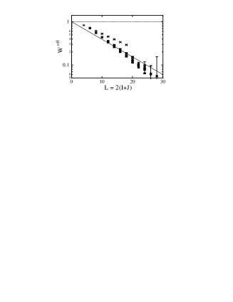
Fig. 1: The comparison between the lattice data and the analytical estimation of $W_{C}^{\rm off}$ $\equiv$ $\langle W_{C}[U_{\mathchar 28950\relax}(\cdot)]\rangle/\langle W_{C}[u_{\mathchar 28950\relax}(\cdot)]\rangle$ as the function of the perimeter $L\equiv 2(I+J)$ in the MA gauge. The cross ($\times$) denotes the lattice date at $\mathchar 28940\relax=2.4$, and the straight line denotes the theoretical estimation of $W_{C}^{\rm off}=\exp\{L\langle\ln(\cos\mathchar 28946\relax_{\mathchar 28950\relax}(s))\rangle_{\rm MA}\}$ with the microscopic input $\langle\ln\{\cos\mathchar 28946\relax_{\mathchar 28950\relax}(s)\}\rangle_{\rm MA}\simeq-0.082$ at $\mathchar 28940\relax=2.4$. The off-diagonal gluon contribution $W_{C}^{\rm off}$ seems to obey the perimeter law for $I,J\geq 2$ (thick cross symbols).

5 Origin of Abelian Dominance : Effective Charged-Gluon Mass induced in MA Gauge

In the MA gauge, only the diagonal gluon component is relevant for the infrared quantities like the string tension and the chiral condensate, and it is regarded as abelian dominance for NP-QCD. In this section, we study the origin of abelian dominance in the MA gauge.

As a possible physical interpretation, abelian dominance can be expressed as generation of the effective mass $m_{ch}$ of the off-diagonal (charged) gluon by the MA gauge fixing in the QCD partition functional,²

$$Z_{\rm QCD}^{\rm MA} = \int DA_{\mathchar 28950\relax}\exp\{iS_{\rm QCD}[A_{\mathchar 28950\relax}]\}\mathchar 28942\relax(\mathchar 28936\relax_{\rm MA}^{\pm}[A_{\mathchar 28950\relax}])\mathchar 28929\relax_{\rm PF}[A_{\mathchar 28950\relax}]$$ (5.1)

$$\simeq \int DA_{\mathchar 28950\relax}^{3}\exp\{iS_{\rm eff}[A_{\mathchar 28950\relax}^{3}]\}\int DA_{\mathchar 28950\relax}^{\pm}\exp\{i\int d^{4}x\ m_{ch}^{2}A_{\mathchar 28950\relax}^{+}A^{\mathchar 28950\relax}_{-}\}{\cal F}[A_{\mathchar 28950\relax}],$$ (5.2)

where $\mathchar 28929\relax_{\rm FP}$ is the Faddeev-Popov determinant, $S_{\rm eff}[A_{\mathchar 28950\relax}^{3}]$ the abelian effective action and ${\cal F}[A_{\mathchar 28950\relax}]$ a smooth functional. In fact, if the MA gauge fixing induces the effective mass $m_{ch}$ of off-diagonal (charged) gluons, the charged gluon propagation is limited within the short-range region as $r\mathop{{}^{<}}_{\!\!\!\!\!\sim}m_{ch}^{-1}$, and hence off-diagonal gluons cannot contribute to the long-distance physics in the MA gauge, which provides the origin of abelian dominance for NP-QCD.

Here, using the SU(2) lattice QCD in the Euclidean metric, we study the gluon propagator $G_{\mathchar 28950\relax\mathchar 28951\relax}^{ab}(x-y)\equiv\langle A_{\mathchar 28950\relax}^{a}(x)A_{\mathchar 28951\relax}^{b}(y)\rangle$ in the MA gauge with respect to the interaction range and strength.^2,19 As for the residual U(1) gauge symmetry, we impose the U(1) Landau gauge fixing to extract most continuous gauge configuration and to compare with the continuum theory. In particular, the scalar combination $G_{\mathchar 28950\relax\mathchar 28950\relax}^{a}(r)\equiv\sum^{4}_{\mathchar 28950\relax=1}\langle A_{\mathchar 28950\relax}^{~{}a}(r)A_{\mathchar 28950\relax}^{~{}a}(0)\rangle~{}(a=1,2,3)$ is useful to observe the interaction range of the gluon, because it depends only on the four-dimensional Euclidean radial coordinate $r\equiv(x_{\mathchar 28950\relax}x_{\mathchar 28950\relax})^{{1\over 2}}~{}$.

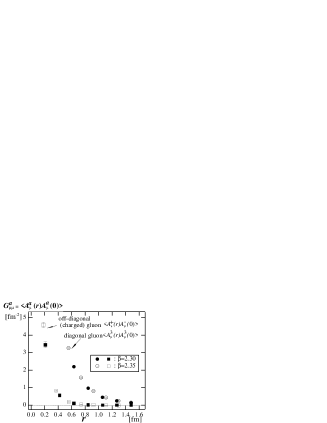
(a)

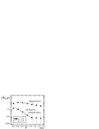
(b)

Fig. 2: (a) The scalar correlation $G_{\mathchar 28950\relax\mathchar 28950\relax}^{a}(r)$ of the gluon propagator as the function of the 4-dimensional distance $r$ in the MA gauge in the SU(2) lattice QCD with $12^{3}\times 24$ and $\mathchar 28940\relax=2.3,2.35.$ In the MA gauge, the off-diagonal (charged) gluon propagates within the short-range region $r\mathop{{}^{<}}_{\!\!\!\!\!\sim}0.4$ fm, and cannot contribute to the long-range physics. (b) The logarithmic plot for the scalar correlation $r^{2}G_{\mathchar 28950\relax\mathchar 28950\relax}^{a}(r)$. The charged-gluon propagator behaves as the Yukawa-type function, $G_{\mathchar 28950\relax\mathchar 28950\relax}\sim{\exp(-m_{ch}r)\over r^{2}}$. The effective mass of the charged gluon can be estimated as $m_{ch}\simeq 0.9{\rm GeV}$ from the slope of the dotted line.

We calculate the gluon propagator $G_{\mathchar 28950\relax\mathchar 28950\relax}^{a}(r)$ in the MA gauge using the SU(2) lattice QCD with $12^{3}\times 24$ and $\mathchar 28940\relax=2.3,2.35$. In the MA gauge, the off-diagonal (charged) gluon propagates within the short-range region $r\mathop{{}^{<}}_{\!\!\!\!\!\sim}0.4$ fm, so that it cannot contribute to the long-range physics, although the charged-gluon effect appears at the short distance as $r\mathop{{}^{<}}_{\!\!\!\!\!\sim}0.4$ fm. On the other hand, the diagonal gluon propagates over the long distance and influences the long-range physics. Thus, we find abelian dominance for the gluon propagator : only the diagonal gluon is relevant at the infrared scale in the MA gauge. This is the origin of abelian dominance for the long-distance physics or NP-QCD.^2,19

Since the propagator of the massive gauge boson with mass $M$ behaves as the Yukawa-type function $G_{\mathchar 28950\relax\mathchar 28950\relax}(r)={3\over 4\mathchar 28953\relax^{2}}{1\over r^{2}}\exp(-Mr)$, the effective mass $m_{ch}$ of the charged gluon can be evaluated from the slope of the logarithmic plot of $r^{2}G_{\mathchar 28950\relax\mathchar 28950\relax}^{+-}(r)\sim\exp(-m_{ch}r)$ as shown in Fig.3. The charged gluon behaves as a massive particle at the long distance, $r\mathop{{}^{>}}_{\!\!\!\!\!\sim}0.4$ fm. We obtain the effective mass of the charged gluon as $m_{ch}\simeq 0.9~{}{\rm GeV}$, which provides the critical scale on abelian dominance.

6 Dual Wilson Loop, Inter-Monopole Potential and Evidence of Dual Higgs Mechanism (Monopole Condensation)

In this section, we study the dual Higgs mechanism by monopole condensation in the NP-QCD vacuum in the field-theoretical manner. Since QCD is described by the “electric variable” as quarks and gluons, the “electric sector” of QCD has been well studied with the Wilson loop or the inter-quark potential, however, the “magnetic sector” of QCD is hidden and still unclear. To investigate the magnetic sector directly, it is useful to introduce the “dual (magnetic) variable” as the dual gluon $B_{\mathchar 28950\relax}$, similarly in the dual Ginzburg-Landau (DGL) theory.^4,5,20-24 The dual gluon $B_{\mathchar 28950\relax}$ is the dual partner of the abelian gluon and directly couples with the magnetic current $k_{\mathchar 28950\relax}$. In particular, in the absence of the electric current, $\partial_{\mathchar 28950\relax}F^{\mathchar 28950\relax\mathchar 28951\relax}=j^{\mathchar 28951\relax}=0$, the dual gluon $B_{\mathchar 28950\relax}$ can be introduced as the regular field satisfying $\partial_{\mathchar 28950\relax}B_{\mathchar 28951\relax}-\partial_{\mathchar 28951\relax}B_{\mathchar 28950\relax}={{}^{*}\!F}_{\mathchar 28950\relax\mathchar 28951\relax}$ and the dual Bianchi identity, ${\partial^{\mathchar 28950\relax}}{{}^{*}\!(}\partial\land B)_{\mathchar 28950\relax\mathchar 28951\relax}=0,$ and therefore the argument on monopole condensation becomes transparent.^20,23

As was mentioned in Section 3, the monopole part in the MA gauge and does not include the electric current, $j_{\mathchar 28950\relax}\simeq 0$, and holds the essence of NP-QCD, which is of interest. Then, it is wise to consider the monopole part for the transparent argument on the dual Higgs mechanism or monopole condensation. In terms of the dual Higgs mechanism, the inter-monopole potential is expected to be short-range Yukawa-type, and the dual gluon $B_{\mathchar 28950\relax}$ becomes massive in the monopole-condensed vacuum.^4,5,20 We define the dual Wilson loop $W_{D}$ as the line-integral of the dual gluon $B_{\mathchar 28950\relax}$ along a loop $C$,

$$W_{D}(C)\equiv\exp\{i{e\over 2}\oint_{C}dx_{\mathchar 28950\relax}B^{\mathchar 28950\relax}\}=\exp\{i{e\over 2}\int\!\!\!\int d\mathchar 28955\relax_{\mathchar 28950\relax\mathchar 28951\relax}{{}^{*}\!F}^{\mathchar 28950\relax\mathchar 28951\relax}\},$$ (6.1)

which is the dual version of the abelian Wilson loop $W_{\rm Abel}(C)\equiv\exp\{i{e\over 2}\oint_{C}dx_{\mathchar 28950\relax}A^{\mathchar 28950\relax}\}=\exp\{i{e\over 2}\int\!\!\!\int d\mathchar 28955\relax_{\mathchar 28950\relax\mathchar 28951\relax}{F}^{\mathchar 28950\relax\mathchar 28951\relax}\}$ in the SU(2) case.²⁵ Here, we have set the test monopole charge as $e/2$ considering this duality correspondence. The potential between the monopole and the anti-monopole is derived from the dual Wilson loop as

$$V_{M}(R)=-\lim_{T\rightarrow\infty}{1\over T}\ln\langle W_{D}(R,T)\rangle.$$ (6.2)

Using the SU(2) lattice QCD in the MA gauge, we study the dual Wilson loop and the inter-monopole potential in the monopole part.²⁵ The dual Wilson loop $\langle W_{D}(I,J)\rangle$ seems to obey the perimeter law rather than the area law for $I,J\geq 2$. The inter-monopole potential is short ranged and flat in comparison with the inter-quark potential as shown in Fig.4.

At the long distance, the inter-monopole potential can be fitted by the simple Yukawa potential $V_{M}(r)=-{{(e/2)}^{2}\over 4\mathchar 28953\relax}{e^{-m_{B}r}\over r}$. The dual gluon mass is estimated as $m_{B}\simeq{\rm 0.5GeV}$, which is consistent with the DGL theory.^4,5,20-23 The mass generation of the dual gluon $B_{\mathchar 28950\relax}$ would provide the direct evidence of the dual Higgs mechanism by monopole condensation at the infrared scale in the NP-QCD vacuum.

In the whole region of $r$ including the short distance, the inter-monopole potential seems to be fitted by the Yukawa-type potential with the effective size $R$ of the QCD-monopole as shown in Fig.4.

(a)

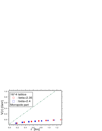
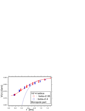
(b)

Fig. 3: (a) The dual Wilson loop $\langle W_{D}(I,J)\rangle$ v.s. its area $(I\times J)$ and its perimeter $2(I+J)$ in the monopole part in the MA gauge in the SU(2) lattice QCD with $16^{4}$ and $\mathchar 28940\relax=2.35$. $\langle W_{D}(I,J)\rangle$ seems to obey the perimeter law rather than the area law for $I,J\geq 2$ (thick cross symbols). (b) The inter-monopole potential $V_{M}(r)$ in the monopole part in the MA gauge extracted from $\langle W_{D}(I,J)\rangle$. $r$ is the 3-dimensional distance between the monopole and the anti-monopole. The dashed-dotted line denotes the linear part of the inter-quark potential in the left figure. In the right figure, the dashed curve and the solid curve denote the simple Yukawa potential and the Yukawa-type potential with the effective monopole size, respectively.

The fitting on the global shape of $V_{M}(r)$ suggests the dual gluon mass as $m_{B}\simeq 0.5{\rm GeV}$ and the effective monopole size $R\simeq 0.35{\rm fm}$, which would provide the critical scale for NP-QCD in terms of the dual Higgs theory as the local field theory.

7 Origin of Strong Correlation between Monopoles and Instantons : Large Gluon-Field Fluctuation around Monopoles

There is no point-like monopole in QED, because the QED action diverges around the monopole. The QCD-monopole also accompanies the large fluctuation of the abelian action density inevitably. In this section, we study the action density around the QCD-monopole in the MA gauge using the SU(2) lattice QCD.²⁶

From the SU(2) plaquette $P^{\rm SU(2)}_{\mathchar 28950\relax\mathchar 28951\relax}(s)$ and the abelian plaquette $P^{\rm Abel}_{\mathchar 28950\relax\mathchar 28951\relax}(s)$, we define the “SU(2) action density” $S_{\mathchar 28950\relax\mathchar 28951\relax}^{\rm SU(2)}(s)\equiv 1-{1\over 2}{\rm tr}P^{\rm SU(2)}_{\mathchar 28950\relax\mathchar 28951\relax}(s),$ the “abelian action density” $S_{\mathchar 28950\relax\mathchar 28951\relax}^{\rm Abel}(s)\equiv 1-{1\over 2}{\rm tr}P^{\rm Abel}_{\mathchar 28950\relax\mathchar 28951\relax}(s)$ and the “off-diagonal action density”

$$S_{\mathchar 28950\relax\mathchar 28951\relax}^{\rm off}(s)\equiv S_{\mathchar 28950\relax\mathchar 28951\relax}^{\rm SU(2)}(s)-S_{\mathchar 28950\relax\mathchar 28951\relax}^{\rm Abel}(s),$$ (7.1)

which is not positive definite. In the lattice formalism, the monopole current $k_{\mathchar 28950\relax}(s)$ is defined on the dual link, and there are 12 links around the monopole. To investigate the “local quantity around the monopole”, we define the “local average over the neighboring 12 links around the dual link”,

$$\bar{S}(s,\mathchar 28950\relax)\equiv{1\over 12}\sum_{\mathchar 28939\relax\mathchar 28940\relax\mathchar 28941\relax}\sum_{m=0}^{1}|\mathchar 28962\relax_{\mathchar 28950\relax\mathchar 28939\relax\mathchar 28940\relax\mathchar 28941\relax}|S_{\mathchar 28939\relax\mathchar 28940\relax}(s+m\hat{\mathchar 28941\relax}).$$ (7.2)

From the total ensemble $\{\bar{S}(s,\mathchar 28950\relax)\}_{s,\mathchar 28950\relax}$, we extract the sub-ensemble $\{\bar{S}(s,\mathchar 28950\relax)\}_{s,\mathchar 28950\relax}$ around the monopole in the lattice QCD. We show in Fig.5(b) the probability distribution of $\bar{S}_{\rm SU(2)}$, $\bar{S}_{\rm Abel}$ and $\bar{S}_{\rm off}$ around the monopole in the MA gauge.

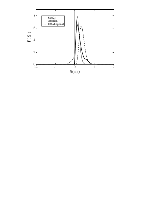
(a)

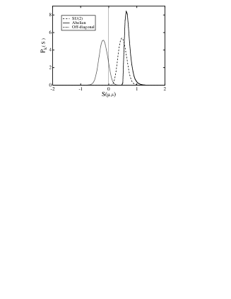
(b)

Fig. 4: (a) The total probability distribution $P(\bar{S})$ and (b) The probability distribution $P_{k}(\bar{S})$ around the monopole for SU(2) action density $\bar{S}_{\rm SU(2)}$ (dashed curve), abelian action density $\bar{S}_{\rm Abel}$ (solid curve) and off-diagonal part $\bar{S}_{\rm off}$ (dotted curve) in the MA gauge at $\mathchar 28940\relax=2.4$ on $16^{4}$ lattice. Large cancellation between $\bar{S}_{\rm Abel}$ and $\bar{S}_{\rm off}$ is observed around the QCD-monopole.

Around the monopole in the MA gauge, a large fluctuation is observed both in $S_{\rm Abel}$ and in $S_{\rm off}$, however, the total QCD action $\bar{S}_{\rm SU(2)}$ is kept to be small relatively, owing to large cancellation between $\bar{S}_{\rm Abel}$ and $\bar{S}_{\rm off}$ as shown in Fig.5(b).²⁶ Thus, off-diagonal gluons play the essential role to appearance of QCD-monopoles to keep the total QCD action finite. However, in the infrared scale, off-diagonal gluons become irrelevant, while large abelian-gluon fluctuations originated from QCD-monopoles remain to be relevant in the MA gauge.

Even in the MA gauge, off-diagonal gluons largely remain around the QCD-monopole, which would provide the effective monopole size $R$ as the critical scale of abelian projected QCD (AP-QCD), because off-diagonal gluons become visible and AP-QCD should be modified at the shorter scale than $R$, which resembles the structure of the ’t Hooft-Polyakov monopole. The concentration of off-diagonal gluons around monopoles leads to the local correlation between monopoles and instantons: instantons appear around the monopole world-line in the MA gauge, because instantons need full SU(2) gluon components for existence.^{7,8,13-15,23,24,27-29}

One of the authors (H.S.) would like to thank Professor Y. Nambu for his useful comments and discussions. The authors would like to thank Prof. O. Miyamura, Dr. S. Sasaki and all the members of RCNP theory group for useful discussions.

References

[1]
Y. Nambu, Phys. Rev.D10, 4262 (1974).
[2]
H. Suganuma, K. Amemiya, A. Tanaka and H. Ichie,
Proc. of Innovative Computational Methods
in Nuclear Many-Body Problems (INNOCOM ’97) (World Scientific).
[3]
G. ’t Hooft, Nucl. Phys.B190, 455 (1981).
[4]
H. Suganuma, S. Sasaki and H. Toki,
Nucl. Phys.B435, 207 (1995) and references.
[5]
H. Suganuma, S. Sasaki, H. Toki and H. Ichie,
Prog. Theor. Phys. (Suppl.)120, 57 (1995).
[6]
Z. F. Ezawa and A. Iwazaki, Phys. Rev.D25,
2681 ; D26, 631 (1982).
[7]
H. Suganuma, M. Fukushima, H. Ichie and A. Tanaka,
Nucl. Phys.B (Proc. Suppl.) 65, 29 (1998).
[8]
H. Suganuma, A. Tanaka, S. Sasaki and O. Miyamura,
Nucl. Phys.B (Proc.Suppl.) 47, 302 (1996).
[9]
A. S. Kronfeld, G. Schierholz
and U.-J. Wiese,
Nucl. Phys.B293, 461 (1987).
[10]
T. Suzuki and I. Yotsuyanagi, Phys. Rev.D42, 4257 (1990).
[11]
S. Hioki, S. Kitahara, S. Kiura, Y. Matsubara,
O. Miyamura, S. Ohno and T. Suzuki,
Phys. Lett.B272, 326 (1991).
[12]
O. Miyamura, Phys. Lett.B353, 91 (1995).
[13]
H. Suganuma, S. Sasaki, H. Ichie, F. Araki and O. Miyamura,
Nucl. Phys.B (Proc.Suppl.) 53, 524 (1997).
[14]
H. Suganuma, S. Umisedo, S. Sasaki, H. Toki and O. Miyamura,
Aust. J. Phys.50, 233 (1997).
[15]
M. Polikarpov, Nucl. Phys.B (Proc.Suppl.)
53, 134 (1997) and references.
[16]
R. Woloshyn, Phys. Rev.D51, 6411 (1995).
[17]
A. Di Giacomo, Nucl. Phys.B (Proc.Suppl.)
47, 136 (1996) and references.
[18]
T. DeGrand and D. Toussaint, Phys. Rev.D22, 2478 (1980).
[19]
K. Amemiya and H. Suganuma,
Proc. of INNOCOM ’97 (World Scientific).
[20]
H. Ichie, H. Suganuma and H. Toki,
Phys. Rev.D54, 3382 (1996); D52, 2994 (1995).
[21]
S. Sasaki, H. Suganuma and H. Toki,
Phys. Lett.B387, 145 (1996).
[22]
S. Umisedo, H. Suganuma and H. Toki,
Phys. Rev.D57, 1605 (1998).
[23]
H. Suganuma, S. Sasaki, H. Ichie, H. Toki
and F. Araki, Int. Symp. on Frontier ’96
(World Scientific, 1996) 177.
[24]
H. Suganuma, H. Ichie, S. Sasaki and H. Toki,
Color Confinement and Hadrons (Confinement ’95)
(World Scientific, 1995) 65.
[25]
A. Tanaka and H. Suganuma,
Proc. of INNOCOM ’97 (World Scientific).
[26]
H. Ichie and H. Suganuma,
Proc. of INNOCOM ’97 (World Scientific).
[27]
S. Thurner, H. Markum and W. Sakuler,
Confinement ’95 (World Scientific,1995) 77.
[28]
A. Hart and M. Teper, Phys. Lett.B371,
261 (1996).
[29]
M. Fukushima, S. Sasaki, H. Suganuma, A. Tanaka,
H. Toki and D. Diakonov,
Phys. Lett.B399, 141 (1997).