Perturbative and non-perturbative studies of the SU(2)-Higgs model
on lattices with asymmetric lattice spacings

Abstract

We present a calculation of the ${\cal O}(g^{2},\lambda)$ perturbative corrections to the coupling anisotropies of the SU(2)-Higgs model on lattices with asymmetric lattice spacings. These corrections are obtained by a one-loop calculation requiring the rotational invariance of the gauge and Higgs boson propagators in the continuum limit. The coupling anisotropies are also determined from numerical simulations of the model on appropriate lattices. The one-loop perturbation theory and the simulation results agree with high accuracy. It is demonstrated that rotational invariance is also restored for the static potential determined from space–space and space–time Wilson loops.

PACS Numbers: 11.15.Ha, 12.15.-y

I Introduction

At high temperatures the electroweak symmetry is restored. Since the baryon violating processes are unsuppressed at high temperatures, the observed baryon asymmetry of the universe has finally been determined at the electroweak phase transition [1].

In recent years quantitative studies of the electroweak phase transition have been carried out by means of resummed perturbation theory and lattice Monte Carlo simulations [2]–[17]. In the SU(2)-Higgs model for Higgs masses ($m_{H}$) below 50 GeV, the phase transition is predicted by the perturbation theory to be of first order. However, it is difficult to give a definite perturbative statement for physically more interesting masses, e.g. $m_{H}>80$ GeV. Due to the bad infrared properties of the theory, the perturbative approach breaks down in this parameter region. A systematic and fully controllable treatment is necessary, which can be achieved by lattice simulations.

For smaller Higgs boson masses ($m_{H}<50$ GeV) the phase transition is quite strong and relatively easy to study on the lattice. For larger $m_{H}$ (e.g. $m_{H}=80$ GeV) the phase transition gets weaker, the lowest excitations have masses small compared to the temperature, $T$. From this feature one expects that a finite temperature simulation on an isotropic lattice would need several hundred lattice points in the spatial directions even for $L_{t}=2$ temporal extension. These kinds of lattice sizes are out of the scope of the present numerical resources.

One possibility to solve the problem of these different scales is to integrate out the heavy, ${\cal O}(T)$ modes perturbatively, and analyse the obtained theory on the lattice. This strategy turned out to be quite successful, and both its perturbative and lattice features have been studied by several groups [6]–[11]. Even more: [18] predicts that somewhere above 80 GeV Higgs mass the first order phase transition does not take place any further, the two phases can be continuously connected. Ref. [19] gives estimates of the end-point of the phase transition in the framework of the reduced 3-d approach.

With this paper we follow another approach (analytic and Monte Carlo) to handle this two-scale problem. We will use the simple idea that finite temperature field theory can be conveniently studied on asymmetric lattices, i.e. lattices with different spacings in temporal ($a_{t}$) and spatial ($a_{s}$) directions. This method solves the two-scale problem in a natural way [20]. Another advantage is, well-known and used in QCD, that this formulation makes an independent variation of the temperature ($T$) and volume ($V$) possible. The perturbative corrections to the coupling anisotropies are known in QCD (see refs. [21, 22]). Performing a similar analysis for the SU(2)-Higgs model, we have presented in our earlier paper [23] the perturbative corrections to the coupling anisotropies for this case, too. Here we give details of the perturbative calculation of [23] and by numerical simulation on lattices with anisotropic lattice spacings calculate the coupling asymmetries for the practically reasonable parameters of the SU(2)-Higgs model. As we will show at $m_{H}\approx 80$ GeV the one-loop perturbative and the non–perturbative coupling asymmetries agree very well.

There is an essential difference between pure gauge theories and the SU(2)-Higgs model. In the former case any value (within a certain range) of the space and time coupling constant ratio does correspond to a meaningful theory, the actual value of the ratio corresponds to a definite value of the ratio of the space and time lattice spacings. On the other hand, in case of the SU(2)-Higgs model for a fixed value of the space and time gauge coupling ratio (determining the ratio of the space and time lattice spacings) one has to fix the ratio of the space and time hopping parameters to a definite value, in order to ensure that the theory makes sense. A convenient way to do this is to require that the ratio of space and time gauge boson masses should be equal to the ratio of space and time Higgs boson masses. Such a choice of the parameters is a precondition to both the perturbative calculations and the numerical simulations.

The plan of this paper is as follows. Section II. deals with the perturbative analysis. In subsection II.A we give the lattice action of the model on asymmetric lattices and discuss perturbation theory in the anisotropic lattice case. Subsection II.B contains the calculation of the critical hopping parameter and of the wave function quantum correction terms, which give the quantum corrections to the anisotropy parameters. In subsection II.C a discussion of the finite temperature continuum limit is given. The optimal choice of the ratio of space and time lattice spacings is determined by perturbative techniques. Section III. contains our non-perturbative analysis. Subsection III.A gives the basic points of our MC simulations. Subsection III.B deals with the mass determinations from the correlation functions. In subsection III.C we present the results on Wilson loop simulations and the static potential. In subsection III.D we finally evaluate the non-perturbative asymmetries and compare them with the perturbative results. Section IV. is a summary and outlook.

II Lattice action and perturbation theory

In this section we discuss lattice perturbation theory. Since we did not find the Feynman rules for the anisotropic lattice spacing case in the literature, we present some details of lattice perturbation theory. After that we determine the critical hopping parameter and the anisotropies in one-loop perturbation theory. The continuum limit and the optimal choice of the ratio of space- and time-like lattice spacings is also discussed.

A Action in continuum notation, gauge fixing, propagators

For simplicity, we use equal lattice spacings in the three spatial directions ($a_{i}=a_{s},\ i=1,2,3$) and another spacing in the temporal direction ($a_{4}=a_{t}$). The asymmetry of the lattice spacings is characterized by the asymmetry factor $\xi=a_{s}/a_{t}$. The different lattice spacings can be ensured by different coupling strengths in the action for time-like and space-like directions. The action reads

$$S[U,\varphi] = \beta_{s}\sum_{sp}\left(1-{1\over 2}{\rm Tr\,}U_{sp}\right)+\beta_{t}\sum_{tp}\left(1-{1\over 2}{\rm Tr\,}U_{tp}\right)$$ (3)

$$+\sum_{x\in\Lambda}\left\{{1\over 2}{\rm Tr\,}(\varphi_{x}^{+}\varphi_{x})+\lambda\left[{1\over 2}{\rm Tr\,}(\varphi_{x}^{+}\varphi_{x})-1\right]^{2}\right.$$

$$\left.-\kappa_{s}\sum_{\mu=1}^{3}{\rm Tr\,}(\varphi^{+}_{x+\hat{\mu}}U_{x,\mu}\,\varphi_{x})-\kappa_{t}{\rm Tr\,}(\varphi^{+}_{x+\hat{4}}U_{x,4}\,\varphi_{x})\right\},$$

where $\Lambda$ stands for the lattice points, $U_{x,\mu}$ denotes the SU(2) gauge link variable, $U_{sp}$ and $U_{tp}$ the path-ordered product of the four $U_{x,\mu}$ around a space-space and space-time plaquette, respectively. The symbol $\varphi_{x}$ stands for the Higgs field.

The values of anisotropies defined as

$$\gamma_{\beta}^{2}={\beta_{t}\over\beta_{s}}\ \ \ ,\ \ \ \ \gamma_{\kappa}^{2}={\kappa_{t}\over\kappa_{s}}$$ (4)

are choosen to correspond to given values of the asymmetry $\xi$. In perturbation theory this can be ensured order by order in the loop expansion, requiring that in the limit $a_{s},\,a_{t}\rightarrow 0$ with the ratio $\xi=a_{s}/a_{t}$ fixed, certain physical quantities show rotation symmetry on submanifolds of the bare coupling space satisfying $\gamma_{\beta}=const$, $\gamma_{\kappa}=const$. This procedure leads to a formal double expansion in $g^{2}$ and $\lambda$ of the anisotropies:

$$\gamma_{\beta}^{2}=\xi^{2}\left[1+c_{\beta}(\xi)g^{2}+b_{\beta}(\xi)\lambda+{\cal O}(g^{4},\lambda^{2})\right],\ \ \gamma_{\kappa}^{2}=\xi^{2}\left[1+c_{\kappa}(\xi)g^{2}+b_{\kappa}(\xi)\lambda+{\cal O}(g^{4},\lambda^{2})\right].$$ (5)

Here $g$ is the bare gauge coupling of the theory with symmetric lattice spacings in standard notation. (Note that $c_{\beta}(1)=c_{\kappa}(1)=b_{\beta}(1)=b_{\kappa}(1)=0$.) In this double expansion we use the formal power counting $\lambda\sim g^{2}$. In general, fixing $\gamma_{\beta}(\xi)$ and $\gamma_{\kappa}(\xi)$ to ensure rotation symmetry should be done non-perturbatively. In the non-perturbative framework the definition of $\xi$ is given as the ratio of space and time direction lattice unit correlation lengths. This non-perturbative analysis will be the topic of section III., where we choose the values of the bare copuling ratios (4) to ensure that the Higgs and gauge boson correlation lengths in physical units be the same in the different directions. This idea can be applied in perturbation theory as well (see e.g. [22]), and we will follow this method in our analysis, too.

Elaborating perturbation theory we follow the usual steps (see e.g. [24], [25] for the isotropic SU(2)-Higgs model). The only complication is that we have to keep track of the different lattice spacings and couplings.
First we consider the gauge part of the action. We will use the same notation as applied by the calculation [21] for the pure gauge theory,

$$U_{x,\mu}=\exp\left(ia_{\mu}g_{\mu}\frac{\tau_{r}}{2}A_{\mu}^{r}(x)\right),$$ (6)

where $r$ is summed over 1,2,3, while $\mu$ is not summed, moreover $a_{\mu}=a_{s}$, $g_{\mu}=g_{s}$ for $\mu=1,2,3$ and $a_{4}=a_{t}$, $g_{4}=g_{t}$. We have also

$$\beta_{s}=\frac{4}{\xi}\frac{1}{g_{s}(\xi)^{2}},\ \ \beta_{t}=4\xi\frac{1}{g_{t}(\xi)^{2}}$$ (7)

as the connection to the lattice parameters. The expansions for $g_{s}$, $g_{t}$ read:

$$g_{s}(\xi)^{2}=g^{2}(1-c_{s}(\xi)g^{2}-b_{s}(\xi)\lambda+{\cal O}(g^{4},\lambda^{2})),$$ (8)

$$g_{t}(\xi)^{2}=g^{2}(1+c_{t}(\xi)g^{2}+b_{t}(\xi)\lambda+{\cal O}(g^{4},\lambda^{2})),$$ (9)

where $g^{2}=g_{t}^{2}(\xi=1)=g_{s}^{2}(\xi=1)$ and $c_{\beta}(\xi)=c_{t}(\xi)-c_{s}(\xi)$, $b_{\beta}(\xi)=b_{t}(\xi)-b_{s}(\xi)$.

We write

$$U_{x,\mu}=a_{\mu}^{0}(x)+i\tau_{r}a_{\mu}^{r}(x),$$ (10)

where

$$a_{\mu}^{0}(x)=\cos\left(\frac{a_{\mu}g_{\mu}|A_{\mu}(x)|}{2}\right),\ \ \ a_{\mu}^{r}(x)=\frac{A_{\mu}^{r}(x)}{|A_{\mu}(x)|}\sin\left(\frac{a_{\mu}g_{\mu}|A_{\mu}(x)|}{2}\right),$$ (11)

with $|A_{\mu}(x)|=\sqrt{A_{\mu}^{r}(x)A_{\mu}^{r}(x)}$. The expansion is given by:

$$a_{\mu}^{0}(x)=1-\frac{(a_{\mu}g_{\mu})^{2}}{8}A_{\mu}^{r}A_{\mu}^{r}+\frac{(a_{\mu}g_{\mu})^{4}}{384}A_{\mu}^{r}A_{\mu}^{r}A_{\mu}^{s}A_{\mu}^{s}+{\cal O}(g^{6}),$$ (12)

$$a_{\mu}^{r}(x)=\frac{a_{\mu}g_{\mu}}{2}A_{\mu}^{r}-\frac{(a_{\mu}g_{\mu})^{3}}{48}A_{\mu}^{r}A_{\mu}^{s}A_{\mu}^{s}+{\cal O}(g^{5}).$$ (13)

Inserting eq. (10) into the plaquette parts of the lattice action we get the parts of the action containing odd numbers of gauge boson fields ($S_{pl}^{odd}$) and even numbers of gauge boson fields ($S_{pl}^{even}$). They read:

$$S_{pl}^{odd}=-\sum_{x\in\Lambda}\sum_{\mu<\nu}\beta_{\mu\nu}\left\{\epsilon_{prs}(a_{\nu}^{0}(x+\hat{\mu}a_{\mu})a_{\mu}^{p}(x)+a_{\mu}^{0}(x)a_{\nu}^{p}(x+\hat{\mu}a_{\mu}))a_{\mu}^{r}(x+\hat{\nu}a_{\nu})a_{\nu}^{s}(x)\right.$$ (14)

$$\left.-\epsilon_{prs}a_{\mu}^{p}(x)a_{\nu}^{r}(x+\hat{\mu}a_{\mu})(a_{\nu}^{0}(x)a_{\mu}^{s}(x+\hat{\nu}a_{\nu})+a_{\mu}^{0}(x+\hat{\nu}a_{\nu})a_{\nu}^{s}(x))\right\},$$ (15)

$$S_{pl}^{even}=-\sum_{x\in\Lambda}\sum_{\mu<\nu}\beta_{\mu\nu}\left\{a_{\mu}^{0}(x)a_{\nu}^{0}(x+\hat{\mu}a_{\mu})a_{\mu}^{0}(x+\hat{\nu}a_{\nu})a_{\nu}^{0}(x)-a_{\mu}^{0}(x)a_{\nu}^{0}(x+\hat{\mu}a_{\mu})a_{\mu}^{r}(x+\hat{\nu}a_{\nu})a_{\nu}^{r}(x)\right.$$ (16)

$$\left.-a_{\mu}^{0}(x+\hat{\nu}a_{\nu})a_{\nu}^{0}(x)a_{\mu}^{r}(x)a_{\nu}^{r}(x+\hat{\mu}a_{\mu})+a_{\mu}^{r}(x)a_{\nu}^{r}(x+\hat{\mu}a_{\mu})a_{\nu}^{s}(x+\hat{\nu}a_{\nu})a_{\nu}^{s}(x)\right.$$ (17)

$$\left.+(a_{\nu}^{0}(x+\hat{\mu}a_{\mu})a_{\mu}^{r}(x)+a_{\mu}^{0}(x)a_{\nu}^{r}(x+\hat{\mu}a_{\mu}))(a_{\nu}^{0}(x)a_{\mu}^{r}(x+\hat{\nu}a_{\nu})+a_{\mu}^{0}(x+\hat{\nu}a_{\nu})a_{\nu}^{r}(x))\right.$$ (18)

$$\left.+(-\delta_{ps}\delta_{rt}+\delta_{pt}\delta_{rs})a_{\mu}^{p}(x)a_{\nu}^{r}(x+\hat{\mu}a_{\mu})a_{\mu}^{s}(x+\hat{\nu}a_{\nu})a_{\nu}^{t}(x)\right\},$$ (19)

where p,r,s,t=1,$\ldots,3$ and $\beta_{\mu\nu}$ is equal to $\beta_{s}$ for space indices and equal to $\beta_{t}$ for one space and one time index.

The integration measure for the gauge variables also contributes to the action.

$$d^{3}U_{x,\mu}=\frac{1}{\pi^{2}}d^{4}a_{\mu}^{S}(x)\delta(a_{\mu}^{T}(x)a_{\mu}^{T}(x)-1)$$ (21)

$$\rightarrow d^{3}A_{\mu}^{r}(x)\exp\left(\log\left(\frac{\sin^{2}(\frac{g_{\mu}a_{\mu}}{2}|A_{\mu}|)}{\frac{1}{4}g_{\mu}^{2}a_{\mu}^{2}|A_{\mu}|^{2}}\right)\right),$$ (22)

where capital letters run from 0 to 3 and a sum over T=0,$\ldots,3$ is understood. The contribution to the action reads:

$$S_{m}=-\sum_{x\in\Lambda}\sum_{\mu=1}^{4}\log\left(\frac{\sin^{2}\left(\frac{g_{\mu}a_{\mu}}{2}|A_{\mu}|\right)}{\frac{1}{4}g_{\mu}^{2}a_{\mu}^{2}|A_{\mu}|^{2}}\right)=\sum_{x\in\Lambda}\sum_{\mu=1}^{4}\frac{g_{\mu}^{2}a_{\mu}^{2}}{12}A_{\mu}^{r}(x)A_{\mu}^{r}(x)+{\cal O}(g^{4}).$$ (23)

Next we consider the pure scalar part of the action. Introducing the notation

$$\varphi_{x}=H_{0}(x)+i\tau_{r}\pi_{r}(x),$$ (24)

it reads:

$$S_{H}=\sum_{x}\left\{H_{0}(x)^{2}+\pi_{r}(x)\pi_{r}(x)+\lambda(H_{0}(x)^{2}+\pi_{r}(x)\pi_{r}(x)-1)^{2}\right.$$ (25)

$$\left.-2\kappa_{s}\sum_{\mu=1}^{3}\left(H_{0}(x+\hat{\mu}a_{\mu})H_{0}(x)-\pi_{r}(x+\hat{\mu}a_{\mu})\pi_{r}(x)\right)\right.$$ (26)

$$\left.-2\kappa_{t}(H_{0}(x+\hat{4}a_{4})H_{0}(x)-\pi_{r}(x+\hat{4}a_{4})\pi_{r}(x))\right\}.$$ (27)

Assuming that the $H_{0}$ field has a non-zero vacuum expectation value $v$, we write:

$$H_{0}(x)=H(x)+v.$$ (28)

Moreover we introduce the notations

$$g_{0}=6\lambda\frac{1}{\kappa_{s}^{2}}\frac{a_{t}}{a_{s}},\ \ \ \lambda_{c}=\frac{g_{0}}{24}$$ (29)

and the continuum fields

$$H_{c}(x)=\left(\frac{2\kappa_{s}}{a_{s}a_{t}}\right)^{\frac{1}{2}}H(x),\ \ \ \pi_{c}^{r}(x)=\left(\frac{2\kappa_{s}}{a_{s}a_{t}}\right)^{\frac{1}{2}}\pi^{r}(x),\ \ \ v_{c}=\left(\frac{2\kappa_{s}}{a_{s}a_{t}}\right)^{\frac{1}{2}}v.$$ (30)

Using these we find the scalar part of the action using continuum variables to be

$$S_{H}=a_{s}^{3}a_{t}\sum_{x\in\Lambda}\frac{1}{2}\left\{\sum_{i=1}^{3}(\nabla_{i}H_{c}(x)\nabla_{i}H_{c}(x)+\nabla_{i}\pi_{c}^{r}(x)\nabla_{i}\pi_{c}^{r}(x))\right.$$ (31)

$$\left.+\frac{\gamma_{\kappa}^{2}}{\xi^{2}}(\nabla_{4}H_{c}(x)\nabla_{4}H_{c}(x)+\nabla_{4}\pi_{c}^{r}(x)\nabla_{4}\pi_{c}^{r}(x))\right.$$ (32)

$$\left.+m_{0}^{2}((H_{c}(x)+v_{c})^{2}+\pi_{c}^{r}(x)\pi_{c}^{r}(x))+\frac{g_{0}}{12}((H_{c}(x)+v_{c})^{2}+\pi_{c}^{r}(x)\pi_{c}^{r}(x))^{2}\right\},$$ (33)

where

$$a_{s}^{2}m_{0}^{2}=\frac{1-2\lambda}{\kappa_{s}}-6-2\gamma_{\kappa}^{2},$$ (34)

and

$$\nabla_{\mu}f(x)=\frac{f(x+\hat{\mu}a_{\mu})-f(x)}{a_{\mu}}$$ (35)

is the lattice derivative.

Putting $v_{c}=0$ above corresponds to the symmetric phase, in this case $m_{0}^{2}>0$. Determining $v_{c}$ from the non-trivial minimum of the scalar potential one gets

$$v_{c}^{2}=-\frac{6m_{0}^{2}}{g_{0}}\ \ \ {\rm for}\ \ \ m_{0}^{2}<0.$$ (36)

Introducing $m_{H,0}^{2}=-2m_{0}^{2}$ we obtain finally:

$$S_{H}=a_{s}^{3}a_{t}\sum_{x\in\Lambda}\frac{1}{2}\left\{\sum_{i=1}^{3}(\nabla_{i}H_{c}(x)\nabla_{i}H_{c}(x)+\nabla_{i}\pi_{c}^{r}(x)\nabla_{i}\pi_{c}^{r}(x))\right.$$ (37)

$$\left.+\frac{\gamma_{\kappa}^{2}}{\xi^{2}}(\nabla_{4}H_{c}(x)\nabla_{4}H_{c}(x)+\nabla_{4}\pi_{c}^{r}(x)\nabla_{4}\pi_{c}^{r}(x))\right.$$ (38)

$$\left.+m_{H,0}^{2}H_{c}(x)^{2}+\frac{g_{0}}{12}(H_{c}(x)^{2}+\pi_{c}^{r}(x)\pi_{c}^{r}(x))^{2}+\frac{g_{0}v_{c}}{3}H_{c,0}(x)(H_{c,0}^{2}(x)+\pi_{c}^{r}(x)\pi_{c}^{r}(x))\right\}.$$ (39)

Now we consider the gauge–scalar interaction:

$$S_{i}=\sum_{x\in\Lambda}\left\{-\kappa_{s}\sum_{i=1}^{3}{\rm Tr\,}(\varphi_{x+\hat{i}a_{i}}^{+}(U_{x,i}-1)\varphi_{x})-\kappa_{t}{\rm Tr\,}(\varphi_{x+\hat{4}a_{t}}^{+}(U_{x,4}-1)\varphi_{x})\right\}.$$ (40)

Introducing continuum variables we obtain

$$S_{i}=a_{s}^{3}a_{t}\sum_{x\in\Lambda}\left\{\sum_{i=1}^{3}(a_{i}^{0}(x)-1)\left(-\frac{1}{a_{s}^{2}}\left(v_{c}^{2}+2v_{c}H_{c}(x)+H_{c}(x)H_{c}(x)+\pi_{c}^{r}(x)\pi_{c}^{r}(x)\right)\right.\right.$$ (41)

$$\left.\left.-\frac{v_{c}}{a_{s}}\nabla_{i}H_{c}(x)-\frac{1}{a_{s}}\left(H_{c}(x)\nabla_{i}H_{c}(x)+\pi_{c}^{r}(x)\nabla_{i}\pi_{c}^{r}(x)\right)\right)\right.$$ (42)

$$\left.+\frac{\gamma_{\kappa}^{2}}{\xi^{2}}(a_{4}^{0}(x)-1)\left(-\frac{1}{a_{t}^{2}}\left(v_{c}^{2}+2v_{c}H_{c}(x)+H_{c}(x)H_{c}(x)+\pi_{c}^{r}(x)\pi_{c}^{r}(x)\right)-\frac{v_{c}}{a_{t}}\nabla_{4}H_{c}(x)-\right.\right.$$ (43)

$$\left.\left.\frac{1}{a_{s}}\left(H_{c}(x)\nabla_{4}H_{c}(x)+\pi_{c}^{r}(x)\nabla_{4}\pi_{c}^{r}(x)\right)\right)\right.$$ (44)

$$\left.+\frac{1}{a_{s}}\sum_{i=1}^{3}a_{i}^{r}(x)\left(\epsilon_{rst}\pi_{c}^{s}(x)\nabla_{i}\pi_{c}^{t}(x)+\pi_{c}^{r}(x)\nabla_{i}H_{c}(x)-(H_{c}(x)+v_{c})\nabla_{i}\pi_{c}^{r}(x)\right)\right.$$ (45)

$$\left.+\frac{a_{t}}{a_{s}^{2}}\gamma_{\kappa}^{2}a_{4}^{r}(x)\left(\epsilon_{rst}\pi_{c}^{s}(x)\nabla_{4}\pi_{c}^{t}(x)+\pi_{c}^{r}(x)\nabla_{4}H_{c}(x)-(H_{c}(x)+v_{c})\nabla_{4}\pi_{c}^{r}(x)\right)\right\}.$$ (46)

In perturbation theory the gauge has to be fixed. We use as the gauge fixing function

$$f_{r}(x)=\sum_{i=1}^{3}\frac{a_{i}^{r}(x)-a_{i}^{r}(x-\hat{i}a_{i})}{a_{i}^{2}}+\frac{\gamma_{\kappa}^{2}(a_{4}^{r}(x)-a_{4}^{r}(x-\hat{4}a_{t}))}{a_{t}^{2}}+\frac{\alpha v_{c}g^{2}\pi_{c}^{r}}{4},$$ (47)

which is a lattice version of the well known continuum $R_{\xi}$ gauge fixing function. In eq. (47) $\alpha$ is the gauge parameter. This choice ensures that the mixed second order term in $A_{\mu}^{r}(x)$ and $\pi_{c}^{r}(x)$ will drop out from the sum of the gauge–scalar interaction and the gauge fixing parts of the action. We obtain

$$S_{gf}=-\frac{2}{\alpha g^{2}}a_{s}^{3}a_{t}\sum_{x\in\Lambda}f_{r}(x)f_{r}(x),$$ (48)

$$S_{FP}=a_{s}^{3}a_{t}\sum_{x\in\Lambda}\sum_{i=1}^{3}\left\{\frac{1}{a_{s}^{2}}\left\{(\bar{c}_{r}(x)-\bar{c}_{r}(x+\hat{i}a_{i}))a_{i}^{0}(x)(c_{r}(x)+c_{r}(x+\hat{i}a_{i}))\right.\right.$$ (49)

$$\left.\left.+\epsilon_{rst}(\bar{c}_{r}(x)+\bar{c}_{r}(x+\hat{i}a_{i}))a_{i}^{s}(x)(c_{t}(x)-c_{t}(x+\hat{i}a_{i}))\right\}\right.$$ (50)

$$\left.+\frac{\gamma_{\kappa}^{2}}{\xi^{2}a_{t}^{2}}\left\{(\bar{c}_{r}(x)-\bar{c}_{r}(x+\hat{4}a_{t}))a_{4}^{0}(x)(c_{r}(x)+c_{r}(x+\hat{4}a_{t}))\right.\right.$$ (51)

$$\left.\left.+\epsilon_{rst}(\bar{c}_{r}(x)+\bar{c}_{r}(x+\hat{4}a_{t}))a_{4}^{s}(x)(c_{t}(x)-c_{t}(x+\hat{4}a_{4}))\right\}\right.$$ (52)

$$\left.-\alpha\frac{g^{2}v_{c}}{4}\left\{\bar{c}_{r}(x)c_{r}(x)(H_{c}(x)+v_{c})+\epsilon_{rst}\bar{c}_{r}(x)c_{s}(x)\pi_{c}^{t}(x)\right\}\right\}.$$ (53)

The final form of the continuum notation action reads:

$$S_{cont}=S_{pl}^{odd}+S_{pl}^{even}+S_{m}+S_{H}+S_{i}+S_{gf}+S_{FP},$$ (54)

where the individual terms are given in eqs. (14, LABEL:even, 23, 37, 41, 48, 49). The vertices of perturbation theory may be easily obtained from eq. (54). As usual in lattice perturbation theory we have new vertices proportional to $g^{n}$ for $n\geq 2$.

The formulae to compute the Fourier transforms are as follows. For the gauge field:

$$\tilde{a}_{k,\mu}^{R}=a_{s}^{3}a_{t}\sum_{x\in\Lambda}\exp\left(-i(k,x)-\frac{ia_{\mu}}{2}k_{\mu}\right)a_{\mu}^{R}(x),$$ (55)

where $(k,x)=2\pi(\frac{\nu_{1}l_{1}}{L_{1}}+\cdots+\frac{\nu_{4}l_{4}}{L_{4}})$, $R=0,1,2,3$ and

$$k_{\mu}=\frac{2\pi}{L_{\mu}a_{\mu}}\nu_{\mu},\ \ x_{\mu}=a_{\mu}l_{\mu},$$ (56)

moreover the integers $\nu_{\mu}$, $(l_{\mu})$ take values from $0,1,\dots,L_{\mu}-1$.

The inverse relation is:

$$a_{\mu}^{R}(x)=\frac{1}{L_{1}L_{2}L_{3}L_{4}}\frac{1}{a_{1}a_{2}a_{3}a_{4}}\sum_{\nu_{\mu}}\exp\left(i(k,x)+\frac{ia_{\mu}}{2}k_{\mu}\right)\tilde{a}_{k,\mu}^{R}.$$ (57)

For a lattice infinite in all directions we have

$$a_{\mu}^{R}(x)=\frac{1}{(2\pi)^{4}}\prod_{\rho=1}^{4}\int_{-\pi/a_{\rho}}^{\pi/a_{\rho}}dp_{\rho}\exp\left(ip\cdot x+ip_{\mu}a_{\mu}\right)\tilde{a}_{k,\mu}^{R},$$ (58)

and $p\cdot x=\sum_{\nu=1}^{4}p_{\nu}x_{\nu}$.

For scalar fields we have similar formulae, however, the second terms are missing in the exponents of eqs. (55,57,58).

Our aim is to perform perturbative calculations. The first step is to write down the propagators of the fields from parts quadratic in the fields of the action. We want to determine the tree-level propagators, which are zeroth order in $g$ and $\lambda$. Since $\gamma_{\beta}$ and $\gamma_{\kappa}$ do depend on the couplings, we use $\xi$ in the propagators as their tree-level values. The remaining correction terms from $\gamma_{\beta}$ and $\gamma_{\kappa}$ are quadratic in the fields and give two particle vertices similarly to the measure term in the action in the isotropic case. These will be absorbed by the kinetic parts of the propagators (see later in eqs. (70)–(73)).

The inverse tree-level propagators in momentum space have the following forms.
For the Higgs boson

$$\tilde{\Delta}_{H,0}(p)^{-1}=\sum_{i=1}^{4}{\hat{p}}_{i}^{2}+m_{H,0}^{2},$$ (59)

for the Goldstone bosons

$$\tilde{\Delta}_{\pi_{r}^{c},0}(p)^{-1}=\sum_{i=1}^{4}{\hat{p}}_{i}^{2}-\alpha m_{W,0}^{2},$$ (60)

for the gauge boson

$$\tilde{\Delta}_{W,0,\mu\nu}^{ab}(p)^{-1}=\delta^{ab}\delta_{\mu\nu}\left[m_{W,0}^{2}+\sum_{i=1}^{4}{\hat{p}}_{i}^{2}\right]-{\hat{p}}_{\mu}{\hat{p}}_{\nu}\frac{1+\alpha}{\alpha},$$ (61)

for the ghost

$$\tilde{\Delta}_{FP,0}(p)^{-1}=\sum_{i=1}^{4}{\hat{p}}_{i}^{2}-\alpha m_{W,0}^{2},$$ (62)

where

$${\hat{p}}_{i}={2\over a_{s}}\sin{a_{s}p_{i}\over 2},\ \ \ {\hat{p}}_{4}={2\over a_{t}}\sin{a_{t}p_{4}\over 2}.$$ (63)

The masses have the following expressions in terms of other parameters:

$$m_{H,0}^{2}=-{2\over a_{s}^{2}}\left[{1-2\lambda\over\kappa}\xi-6-2\xi^{2}\right],\ \ \ m_{W,0}^{2}={m_{H,0}^{2}\kappa^{2}\over 2\lambda\xi\beta}=\frac{v_{c}^{2}g^{2}}{4}.$$ (64)

B Critical hopping parameter and anisotropy parameters

The main goal of the paper is to perform a ${\cal O}(g^{2},\lambda)$ analysis of the theory defined by eq. (3). This means first the determination of the mass-counterterms. One wants to tune the bare parameters in a way to ensure that the one-loop renormalized masses are finite in the continuum limit (however, their values in lattice units do vanish, $a_{s}m_{ren}=0$ for $a_{s}\rightarrow 0,\ a_{t}\rightarrow 0,\ \xi=$ fixed). At the same time the vacuum expectation value of the scalar field will be also zero in lattice units ($a_{s}v_{c}=0$), i.e. we are at the phase transition point between the spontaneously broken Higgs phase and the SU(2) symmetric phase. The condition is fulfilled by an appropriate choice of the hopping parameter (critical hopping parameter). The ratios of the couplings ($\gamma_{\beta}$ and $\gamma_{\kappa}$) are still free parameters and can be fixed by two additional conditions. We demand rotational (Lorenz) invariance for the scalar and gauge boson propagators on the one-loop level. This ensures that the propagators with one-loop corrections have the same form in the $z$– and $t$– directions. Clearly, arbitrary couplings for different directions in eq. (3) would not lead to such rotationally invariant two-point functions.

FIG. 1.: Higgs boson self energy graphs. Solid lines stand for Higgs, dashed lines for Goldstone, curly lines for vector bosons and wavy lines denote ghosts.

The most straightforward method to determine the transition point is the use of the effective potential. The condition $d^{2}V_{eff}(\Phi=0)/d\Phi^{2}=0$ gives a simple, gauge invariant expression for the value of the critical hopping parameter, which is exact in the continuum limit. The relevant formulae are given in Landau gauge in [23]. Here we present the general $R_{\xi}$ effective potential:

$$V_{eff}(\Phi)={m_{0}^{2}\over 2}\Phi^{2}+\lambda_{c}\Phi^{4}+\int_{k}\left[{1\over 2}\log({\hat{k}}^{2}+m_{0}^{2}+12\lambda_{c}\Phi^{2})\right.$$ (65)

$$\left.+{24\lambda_{c}\over{16\lambda_{c}-\alpha g^{2}}}\log({\hat{k}}^{2}+m_{0}^{2}+4\lambda_{c}\Phi^{2}-\alpha g^{2}\Phi^{2}/4)\right.$$ (66)

$$\left.+6\log({\hat{k}}^{2}+g^{2}\Phi^{2}/4)+{3\over 2}\log\left(\frac{{\hat{k}}^{2}-\alpha g^{2}\Phi^{2}/4}{{\hat{k}}^{2}+g^{2}\Phi^{2}/4}\right)\right.$$ (67)

$$\left.-{3\over 2}\log({\hat{k}}^{2}-\alpha g^{2}\Phi^{2}/4)\right],$$ (68)

where

$$\int_{k}\equiv{1\over(2\pi)^{4}}\int_{-\pi/a_{s}}^{\pi/a_{s}}d^{3}k\int_{-\pi/a_{t}}^{\pi/a_{t}}dk_{4}.$$ (69)

Alternatively, one may calculate the one-loop corrections to the masses and require that the renormalized masses be zero in lattice units in the limit of zero lattice spacing and fixed $\xi=a_{s}/a_{t}$, as explained above.

First we consider the corrections arising from the two-point interaction vertices. In addition to these there are the one-loop corrections, which we evaluate later on. Including the two-point interaction vertex corrections the momentum squared sums in eqs. (59), (60), (62) modify to

$$\sum_{i=1}^{4}{\hat{p}}_{i}^{2}\longrightarrow\sum_{i=1}^{3}{\hat{p}}_{i}^{2}+\frac{\gamma_{\kappa}^{2}}{\xi^{2}}{\hat{p}}_{4}^{2}$$ (70)

for the Higgs, Goldstone and ghost propagators. The gauge boson inverse propagator becomes more complicated:

$$\tilde{\Delta}_{W,ij}^{ab}(p)^{-1}=\delta^{ab}\left[\delta_{ij}\left(\frac{v_{c}^{2}g_{s}^{2}}{4}+\sum_{i=1}^{3}{\hat{p}}_{i}^{2}+{\gamma_{\beta}^{2}\over\xi^{2}}{\hat{p}}_{4}^{2}\right)-{\hat{p}}_{i}{\hat{p}}_{j}\left(1+\frac{g_{s}^{2}}{\alpha g^{2}}\right)\right],$$ (71)

$$\tilde{\Delta}_{W,i4}^{ab}(p)^{-1}=\tilde{\Delta}_{W,4i}^{ab}(p)^{-1}=-\delta^{ab}{\hat{p}}_{i}{\hat{p}}_{4}\left[\frac{\gamma_{\beta}}{\xi}+\frac{g_{s}g_{t}}{\alpha g^{2}}\frac{\gamma_{\kappa}^{2}}{\xi^{2}}\right],$$ (72)

$$\tilde{\Delta}_{W,44}^{ab}(p)^{-1}=\delta^{ab}\left[\frac{v_{c}^{2}g_{t}^{2}}{4}\frac{\gamma_{\kappa}^{2}}{\xi^{2}}+\sum_{i=1}^{3}{\hat{p}}_{i}^{2}-{\hat{p}}_{4}^{2}\frac{g_{t}^{2}}{\alpha g^{2}}\frac{\gamma_{\kappa}^{4}}{\xi^{4}}\right].$$ (73)

Let us now consider the self-energy corrections to the Higgs mass. The relevant diagrams are shown in figure 1. Evaluating all graphs we obtain at zero Higgs four-momentum, independent of the gauge choosen (i.e. independent on $\alpha$):

$$a_{s}^{2}(m_{H}^{R})^{2}=a_{s}^{2}m_{H}^{2}-\left(2g_{0}+\frac{9}{2}g^{2}\right)J_{1}(\xi,0),$$ (74)

where we used the notation:

$$J_{n}(\xi,ma_{s})=\frac{a_{s}^{4-2n}}{(2\pi)^{4}}\prod_{\rho=1}^{4}\int_{-\pi/a_{\rho}}^{\pi/a_{\rho}}dk_{\rho}{1\over(m^{2}+{\hat{k}}^{2})^{n}}.$$ (75)

Inserting

$$a_{s}^{2}m_{H}^{2}=-2\left(\frac{1-2\lambda}{\kappa}\xi-6-2\xi^{2}\right)$$ (76)

for the one-loop corrected bare mass and using the notation $\lambda=\kappa^{2}g_{0}/(6\xi)=4\kappa^{2}\lambda_{c}/\xi$ together with $a_{s}^{2}(m_{H}^{R})^{2}=0$, we get solving perturbatively for $\kappa$:

$$\kappa_{c}={\xi\over 2(3+\xi^{2})}+{1\over(3+\xi^{2})^{2}}\left[6\xi J_{1}(\xi,0)-{\xi^{2}\over(3+\xi^{2})}\right]\lambda_{c}+{9\xi J_{1}(\xi,0)\over 16(3+\xi^{2})^{2}}g^{2}.$$ (77)

This result coincides with the $d^{2}V_{eff}(\Phi=0)/d\Phi^{2}=0$ condition of eq. (12) of [23]. For the readers’ convenience we plot $J_{1}(\xi,0)$ of eq. (75) in figure 1 as a function of $1/\xi$. For the special case of symmetric lattice spacings, $\xi=1$, our quantum corrections to the critical hopping parameter reproduce the known result of the isotropic SU(2)-Higgs model ([24, 26]). An 8-term Chebishev polynomial approximation with $6\cdot 10^{-6}$ accuracy to the function reads:

$$J_{1}(\xi,0)=0.2276734-0.000175561/\xi-0.1452559/\xi^{2}$$ (78)

$$-0.03593908/\xi^{3}+0.3487585/\xi^{4}-0.4128226/\xi^{5}$$ (79)

$$+0.2187872/\xi^{6}-0.04609285/\xi^{7}.$$ (80)

It is instructive to check that the same result is obtained starting from the symmetric phase perturbation theory, where some graphs are absent and one is lead to

$$0=-a_{s}^{2}m_{0}^{2}-\left(g_{0}+\frac{9}{4}g^{2}\right)J_{1}(\xi,0).$$ (81)

FIG. 2.: The lattice integral $J_{1}(\xi,0)$ (see text) on asymmetric lattices as a function of $1/\xi$.

Let us now consider the self-energy corrections to the gauge boson mass. The relevant diagrams are shown in figure 3. The inverse propagator (eqs. (71)–(73)) at zero momentum has a specific structure, namely

$$\tilde{\Delta}_{W,ij}^{ab}(0)^{-1}=\delta^{ab}\delta_{ij}m_{W}^{2}\frac{g_{s}^{2}}{g^{2}},$$ (82)

$$\tilde{\Delta}_{W,44}^{ab}(0)^{-1}=\delta^{ab}m_{W}^{2}\frac{g_{t}^{2}}{g^{2}}\frac{\gamma_{\kappa}^{2}}{\xi^{2}}.$$ (83)

One therefore has to determine both the diagonal space–space and the time–time components in order to check consistency. Since the bare mass squared turns out to be ${\cal O}(g^{2})$, we may safely put $g_{s}^{2}/g^{2}=g_{t}^{2}/g^{2}=\gamma_{\kappa}^{2}/\xi^{2}=1$ in (82). Finally we obtain, after imposing zero renormalized lattice unit mass squared:

$$a_{s}^{2}m_{W}^{2}=g^{2}\left(\frac{3}{2}+\frac{9}{2}\frac{m_{W}^{2}}{m_{H}^{2}}\right)J_{1}(\xi,0).$$ (84)

Inserting

$$m_{W}^{2}=m_{H}^{2}\frac{3g^{2}}{4g_{0}},$$ (85)

we get back eq. (77) consistently. Again we have checked that (84) holds in all $R_{\xi}$ gauges.

Next we discuss the anisotropy parameters $\gamma_{\beta}$ and $\gamma_{\kappa}$. Following Karsch and Stamatescu [22] we determine them from the requirement of rotational invariance in the continuum limit $a_{s},a_{t}\rightarrow 0$ at fixed $\xi=a_{s}/a_{t}$. In particular we consider the physical particle propagators, which receive quantum corrections

$$\tilde{\Delta}_{H,1}(p)^{-1}=\tilde{\Delta}_{H}(p)^{-1}+\Sigma_{H,1}(p),\ \ \ \tilde{\Delta}_{W,1,\mu\nu}^{ab}(p)^{-1}=\tilde{\Delta}_{W,\mu\nu}^{ab}(p)^{-1}+\Sigma_{W,1,\mu\nu}^{ab}(p),$$ (86)

where $\tilde{\Delta}_{H}(p)^{-1}$ and $\tilde{\Delta}_{W,\mu\nu}$ are the tree-level propagators corrected with the two-point vertices. $\tilde{\Delta}_{H}(p)^{-1}$ is given by

$$\tilde{\Delta}_{H}(p)^{-1}=m_{H,0}^{2}+\sum_{i=1}^{3}{\hat{p}}_{i}^{2}+{\gamma_{\kappa}^{2}\over\xi^{2}}{\hat{p}}_{4}^{2},$$ (87)

while $\tilde{\Delta}_{W,\mu\nu}$ is given by (71)–(73).

FIG. 3.: Vector boson self energy graphs. Solid lines stand for Higgs, dashed lines for Goldstone, curly lines for vector bosons and wavy lines denote ghosts.

The corrections to the anisotropies in the kinetic parts of eqs. (86) should be cancelled by the kinetic parts of the self-energies. For the Higgs boson this can be achieved by requiring

$$1+\frac{1}{2}\frac{\partial^{2}\Sigma_{H,1}(p)}{\partial p_{i}^{2}}\Big{|}_{p=0}=\frac{\gamma_{\kappa}^{2}}{\xi^{2}}+\frac{1}{2}\frac{\partial^{2}\Sigma_{H,1}(p)}{\partial p_{4}^{2}}\Big{|}_{p=0},$$ (88)

where $i=1,2,3$. The graphs contributing are the momentum dependent ones of figure 1.

For the gauge boson there are several possibilities. As a simple one we choose

$$1+\frac{1}{2}\frac{\partial^{2}\Sigma_{W,1,ii}(p)}{\partial p_{j}^{2}}\Big{|}_{p=0}=\frac{\gamma_{\beta}^{2}}{\xi^{2}}+\frac{1}{2}\frac{\partial^{2}\Sigma_{W,1,ii}(p)}{\partial p_{4}^{2}}\Big{|}_{p=0},$$ (89)

where $i\neq j=1,2,3$. This is easily calculated, since only the $\delta_{i,j}$ term of $\tilde{\Delta}_{W,ij}^{ab}(p)^{-1}$ contributes on the left hand side. Not all the self energy graphs contribute, but only those graphs of figure 3, which depend on the momentum.

Our results for infinite lattices are

$$b_{\beta}(\xi)=0,\ \ b_{\kappa}(\xi)=0,$$ (90)

$$c_{\beta}(\xi)=\int_{-\frac{\pi}{a_{s}}}^{\frac{\pi}{a_{s}}}\int_{-\frac{\pi}{a_{s}}}^{\frac{\pi}{a_{s}}}\int_{-\frac{\pi}{a_{s}}}^{\frac{\pi}{a_{s}}}\int_{-\frac{\pi}{a_{t}}}^{\frac{\pi}{a_{t}}}d^{4}q\frac{a_{s}^{2}}{\sum\hat{q}_{\mu}^{2}}\left\{\left[\bigg{(}1-\frac{1}{\xi^{2}}\bigg{)}\frac{3+\cos(q_{1}a_{1})}{4}-\frac{\cos(q_{3}a_{3})-\cos(q_{4}a_{4})}{4}\right]\right.$$ (91)

$$\left.+\frac{1}{a_{s}^{2}\sum\hat{q}_{\mu}^{2}}\left(-\bigg{(}1-\frac{1}{\xi^{2}}\bigg{)}\sin^{2}(q_{1}a_{1})+\frac{9}{2}\cos^{2}(\frac{q_{1}a_{1}}{2})(\cos(q_{3}a_{3})-\cos(q_{4}a_{4}))\right)\right.$$ (92)

$$\left.+\left(\frac{8\sin^{2}(q_{1}a_{1})}{(a_{s}^{2}\sum\hat{q}_{\mu}^{2})^{2}}+\frac{2\cos^{2}(\frac{q_{1}a_{1}}{2})}{a_{s}^{2}\sum\hat{q}_{\mu}^{2}}\right)\left(\frac{\sin^{2}(q_{3}a_{3})-\xi^{2}\sin^{2}(q_{4}a_{4})}{a_{s}^{2}\sum\hat{q}_{\mu}^{2}}-\frac{\cos(q_{3}a_{3})-\cos(q_{4}a_{4})}{2}\right)\right.$$ (93)

$$\left.+\frac{\sin^{2}(q_{1}a_{1})}{(a_{s}^{2}\sum\hat{q}_{\mu}^{2})^{2}}\left(\frac{\sin^{2}(q_{3}a_{3})-\xi^{2}\sin^{2}(q_{4}a_{4})}{a_{s}^{2}\sum\hat{q}_{\mu}^{2}}-\cos(q_{3}a_{3})+\cos(q_{4}a_{4})\right)\right\},$$ (94)

$$c_{\kappa}(\xi)=\frac{3}{4}\int_{-\frac{\pi}{a_{s}}}^{\frac{\pi}{a_{s}}}\int_{-\frac{\pi}{a_{s}}}^{\frac{\pi}{a_{s}}}\int_{-\frac{\pi}{a_{s}}}^{\frac{\pi}{a_{s}}}\int_{-\frac{\pi}{a_{t}}}^{\frac{\pi}{a_{t}}}d^{4}q\frac{a_{s}^{2}}{\sum\hat{q}_{\mu}^{2}}\left\{\bigg{(}1-\frac{1}{\xi^{2}}\bigg{)}\frac{16}{(a_{s}^{2}\sum\hat{q}_{\mu}^{2})^{2}}\left(\xi^{2}\sin^{2}(q_{4}a_{4})-\sin^{2}(q_{1}a_{1})\right)\right\},$$ (95)

where the sums are over $\mu=1,\dots,4$. The above expressions are easily seen to be finite and independent of $a_{s}$ and $a_{t}$. We have also checked that they are gauge independent. The dependence on $\xi$ is plotted in figure 4.

A 6-term Chebishev polynomial approximation with $2\cdot 10^{-5}$ accuracy to the functions reads:

$$c_{\beta}(\xi)=-0.1687249+0.124013/\xi+0.08608489/\xi^{2}$$ (96)

$$-0.04715295/\xi^{3}-0.0002526438/\xi^{4}+0.006038775/\xi^{5},$$ (97)

$$c_{\kappa}(\xi)=-0.05691582-0.0001275536/\xi+0.07582766/\xi^{2}$$ (98)

$$-0.003112956/\xi^{3}-0.0265274/\xi^{4}+0.01085953/\xi^{5}.$$ (99)

We also have to equate $\tilde{\Delta}_{W,1,13}$ and $\tilde{\Delta}_{W,1,14}$:

$$1+\frac{g_{s}^{2}}{\alpha g^{2}}-\frac{\partial^{2}\Sigma_{W,13}}{\partial p_{1}\partial p_{3}}\Big{|}_{p=0}=\frac{\gamma_{\beta}}{\xi}+\frac{g_{s}g_{t}}{\alpha g^{2}}\frac{\gamma_{\kappa}^{2}}{\xi}-\frac{\partial^{2}\Sigma_{W,14}}{\partial p_{1}\partial p_{4}}\Big{|}_{p=0}.$$ (100)

This is a non-trivial constraint, which our previous expressions do satisfy.

FIG. 4.: $c_{\beta}(\xi)$ and $c_{\kappa}(\xi)$ as functions of $1/\xi$.

There are several important features of the anysotropy parameter result, which should be mentioned. a. Masses in the propagators: A consistent perturbative procedure on the lattice determines the bare parameters, for which the renormalized masses vanish, cf. eq. (77). With these bare couplings other quantities, e.g. asymmetry parameters, are determined. However, using the one-loop renormalized masses ($a_{s}m_{H}^{R}=a_{s}m_{W}^{R}=0$) in the propagators instead of the bare ones leads to changes in the results, which are higher order in $g^{2}$ and $\lambda$. Therefore, all our results are given by the integrals with renormalized masses. b. $g^{2}$ and $\lambda$ corrections: In figure 4 we have given only $c_{\beta}(\xi)$ and $c_{\kappa}(\xi)$. As shown by eq. (90) the functions $b_{\beta}(\xi)$ and $b_{\kappa}(\xi)$ vanish, thus there are no corrections of ${\cal O}(\lambda)$ to the anisotropy parameters. It is easy to understand this result qualitatively, since only graphs with two or more scalar self-interaction vertices have non-trivial dependence on the external momentum. This feature is connected with the well-known fact that the $\Phi^{4}$ theory does not have any wave function correction in first order in the scalar self-coupling. It is worth mentioning that there is only one type of two-loop graph (the setting-sun) which should be combined with the one-loop graphs, in order to obtain the whole ${\cal O}(\lambda^{2})$ correction. c. Pure gauge theory: A number of graphs of figure 3 (namely those containing only vector boson and ghost lines) are identical to those of the pure gauge theory. Evaluating the momentum dependent ones from these diagrams, one reproduces the result of ref. [21] (the function $c_{\beta}(\xi)$ of the present paper corresponds to $c_{\tau}(\xi)-c_{\sigma}(\xi)$ of ref. [21]). The most important contribution comes from the self-energy graph with gauge boson four-coupling. Inclusion of the scalar particles gives only small changes. The relative difference between the $c_{\beta}(\xi)$ functions for the pure SU(2) theory and for the SU(2)-Higgs model is typically a few %. d. Quantum corrections to the hopping parameter: The contributions to the hopping parameter come from the momentum dependent graphs of figure 1. This correction has the same sign and order of magnitude than that of the gauge anisotropy parameter; however it is somewhat smaller. It is possible to combine the anisotropies $c_{\beta}^{\prime}(\xi)=c_{\beta}(\xi)-c_{\kappa}(\xi)$. For this choice in the gauge sector and with $\gamma_{\kappa}=\xi$ the rotational invariance can be restored on the one-loop level, choosing the appropriate value for the lattice spacing asymmetry $a_{s}/a_{t}$. Thus, the masses in both directions will be the same. However, the obtained lattice spacing asymmetry will then slightly differ from the original $\xi$. One gets $a_{s}/a_{t}=\xi(1-g^{2}c_{\kappa}(\xi)/2)+{\cal O}(g^{4},\lambda^{2})$.
e. For later use we specify: $c_{\beta}(4)=-0.13308$, $c_{\kappa}(4)=-0.052353$, thus $c_{\beta}^{\prime}(4)=-0.080727$, $\gamma_{\beta}^{\prime}(4)=3.9193$, $a_{s}/a_{t}=4.05235$.
f. Asymmetry parameters away from the critical line: Following the procedure outlined above one may determine the asymmetry parameters away from the critical line. In this case tree-level masses are nonvanishing and are in fact ${\cal O}(1)$. Therefore one has to keep them in the propagator denominators. Thus the final results become more complicated. We do not reproduce the formulae here, only note that numerically the results are very close to the previous case. Thus the asymmetries determined near the critical line are universally applicable.
g. Finite lattice results: The above formulae are valid for infinite lattice sizes, however, replacing the lattice integrals with the appropriate lattice sums, one gets results valid for finite lattices.

C Perturbative study of the continuum limit of the finite temperature theory and optimal choice of the parameter $\xi$

The approach to the continuum limit of the finite temperature theory may be studied in the approximation of one-loop perturbation theory. The relevant physical quantities we study are the ratio of the critical temperature ($T_{c}$) and the Higgs mass and the ratio of the Higgs and vector boson masses. To calculate them in perturbation theory we first determine the bare Higgs mass parameter using the analogue of eq. (74) for a lattice with finite extension ($L_{t}$) in the $t$-direction, i.e. at finite temperature $T=1/(L_{t}a_{t})$, by imposing the condition $a_{s}^{2}(m_{H}^{R})^{2}=0$. This choice corresponds to the lowest point of the metastability region with $T_{c}=1/(L_{t}a_{t})$, i.e. when the derivative of the effective potential at zero field first becomes negative. Using the same bare coupling parameters in the action we next determine the physical Higgs and vector boson masses on a T=0 lattice (i.e. using a lattice with equal (infinite) physical dimensions in space and time directions).

More precisely, the bare quantity $a_{s}^{2}m_{H}^{2}$ is determined from Eq. (74) with $a_{s}^{2}(m_{H}^{R})^{2}=0$, replacing however $J_{1}(\xi,0)$ with $J_{T}(L_{t},\xi,0)$, where

$$J_{T}(L_{t},\xi,ma_{s})=\frac{\xi}{L_{t}}\sum_{n_{t}=0}^{L_{t}-1}\frac{a_{s}}{(2\pi)^{3}}\prod_{\rho=1}^{3}\int_{-\pi/a_{s}}^{\pi/a_{\rho}}dk_{\rho}{1\over(m^{2}+{\hat{k}}^{2})},$$ (101)

and in the denominator $\hat{k}_{4}$ is given by

$$\hat{k}_{4}=\frac{2}{a_{t}}\sin\frac{2\pi n_{t}}{L_{t}}.$$ (102)

(It is straightforward to write down the finite lattice version of eq. (101), too.) The $T=0$ renormalized Higgs mass ($a_{s}m_{H}^{R}$) is then determined from the unmodified eq. (74) using the already known value of the bare parameter $a_{s}^{2}m_{H}^{2}$ and the infinite volume $T=0$ integral $J_{1}(\xi,0)$. Using $T_{c}=1/(a_{t}L_{t})=\xi/(a_{s}L_{t})$ we finally obtain the simple formula for a given $L_{t}$:

$$T_{c}/m_{H}^{R}=\frac{\xi}{L_{t}}\frac{1}{[(2g_{0}+9g^{2}/2)\,(J_{T}(L_{t},\xi,0)-J_{1}(\xi,0))]^{\frac{1}{2}}}.$$ (103)

In the same approximation $(m_{H}^{R}/m_{W}^{R})^{2}$ equals to the tree level value $4g_{0}/(3g^{2})$.

FIG. 5.: Simulation time necessary to reach 0.1% precision determination of $T_{c}$/$m_{H}^{R}$ (normalized to the $\xi=1$ point) versus $1/\xi$.

The result eq. (103) refers to infinitely large lattices (i.e. infinite in both the space-like and time-like directions for the $T=0$ case and infinite in only the space-like direction for the $T\neq 0$ case.) The continuum limit (realized as $L_{t}\rightarrow\infty$) is well defined. In lattice simulations, however, we always have finite lattices. We have to choose minimal lattice volumes large enough to ensure a reasonable precision. This choice of course does depend on $\xi$, therefore we may also look for the optimal choice of $\xi$ ensuring a reasonable precision (say 0.1%) of the physical mass determinations using the smallest possible lattices or shortest simulation times. This problem may be studied in lattice perturbation theory.

To obtain the optimal choice of $\xi$ we first determine the $L_{t}\rightarrow\infty$ (i.e. the continuum) limit value of $T_{c}/m_{H}^{R}$ as a function of $\xi$ using eq. (103). We obtain that – as expected – the limit of $T_{c}/m_{H}^{R}$ does not depend on $\xi$ within errors.

Next we take into account that in practice we simulate on lattices with finite extensions. In order to fit in the relevant modes we have to deal with a given physical volume:

$$V_{phys}=L_{t}a_{t}(L_{s}\xi a_{t})^{3}={1\over T}(L_{s}/L_{t}\cdot\xi/T)^{3}.$$ (104)

Thus the number of the lattice points (which determines the memory required) is expressed as

$$L_{t}L_{s}^{3}=V_{phys}T^{4}L_{t}^{4}/\xi^{3}.$$ (105)

To get a correct estimate of the simulation time we have to take into account the autocorrelation times as well. Since these are proportional to the squares of the correlation lengths for a local updating algorithm (see [27]), i.e. to $(L_{t}/\xi)^{2}$, the time necessary for simulation on a given physical volume and temperature will be proportional to

$$V_{phys}T^{4}L_{t}^{6}/\xi^{5}.$$ (106)

Next we choose a lattice extension in temporal direction $\bar{L_{t}}$ so that by eq. (103) we obtain an approximation of the previously determined continuum limit $T_{c}/m_{H}^{R}$ value to a given (say 0.1%) precision. $T_{c}/m_{H}^{R}$ as determined from eq. (103) as a function of $L_{t}$ approaches the limiting value from below for large $L_{t}$ for all $\xi$ values. However, for $\xi\geq 2$ it decreases for increasing, small $L_{t}$ values. Thus specific small $L_{t}$ values may better approximate the limiting value of $T_{c}/m_{H}^{R}$ than larger intermediate values. It is clear that this is an accidental agreement only, therefore in our considerations we have determined the smallest $\bar{L_{t}}$ value giving $T_{c}/m_{H}^{R}$ with the required precision, which does not deteriorate for larger $L_{t}$.

More precisely we compare the true continuum limit of $T_{c}/m_{H}^{R}$ with an approximate value obtained from an extrapolation to $L_{t}=\infty$ of the $T_{c}/m_{H}^{R}$ values determined from four subsequent $L_{t}$ values. We choose $\bar{L_{t}}$ to be the minimal $L_{t}$, which (together with the 3 larger $L_{t}$ values) already gives the required precision. Having determined $\bar{L_{t}}$ we calculate the corresponding simulation time for finite lattice size using eq. (106). Figure 5 shows the simulation time normalized to the $\xi=1$ value as a function of $1/\xi$ for 0.1% precision in $T_{c}/m_{H}^{R}$. The normalized simulation time as a function of $\xi$ has a broad minimum near $\xi=2$. The number of lattice points (105) (normalized to the $\xi=1$ value) is quite a similar function of $\xi$ with a broad minimum near $\xi=2$. In our numerical simulations we have choosen $\xi\simeq 4$, which is a good choice both from the point of view of simulation time and fiting in the relevant modes into a practically accessible lattice.

III Non-perturbative analysis of the anisotropies

This section of the paper deals with our non-perturbative determination of the anisotropy parameters by means of numerical simulations. Besides a mere confirmation of the one-loop calculations in the previous part, it could give estimates of possible corrections, which go beyond perturbation theory. This is an important step towards future studies of the finite temperature electroweak phase transition in the framework of the four-dimensional SU(2)-Higgs model on anisotropic lattices. Namely, if the deviation from the perturbative results turns out to be so small that its influence on expectation values in a numerical simulation is negligible within their typical statistical errors, the one-loop perturbative anisotropies $\gamma_{\beta}$, $\gamma_{\kappa}$ and $\xi$ can be used without any further (non-perturbative) fine-tuning. At first sight this may not seem very surprising, because the zero-temperature theory is weakly coupled ($g^{2}\simeq 0.5$). But owing to the fact that the corrections in the parameter $\lambda$ — entering only at two-loop level — whose size essentially determines the value of the Higgs boson mass, are not exactly known, such an investigation is necessary, particularly in view of Higgs masses around 80 GeV or larger, which is the physically allowed region determined by the LEP experiments.

As already discussed above, the tree-level values of the anisotropies receive quantum corrections, which in general have to be determined non-perturbatively. A physically motivated idea for their estimation is to impose the restoration of the space-time interchange symmetry as a remnant of Lorentz invariance after discretization of the continuum theory. In practice this is to be realized by the requirement that Higgs and gauge boson correlation lengths in physical units should be equal in space- and time-like directions. Furthermore, we include into the analysis the length scale of the static potential derived from space-time and space-space Wilson loops.

The following subsections describe our numerical studies in more detail. After some brief remarks on the simulation techniques and parameters used, we present the results on the physical observables under consideration and propose, how they can serve to extract the coupling and lattice spacing anisotropies non-perturbatively. Finally, the values obtained in this way are confronted with perturbation theory.

A Monte Carlo simulation and its parameters

In our Monte Carlo simulations we apply an optimized combination of heatbath and overrelaxation algorithms, which has been extensively discussed for the isotropic model in refs. [13, 14, 28], and their implication carries over straightforwardly to an anisotropic lattice. The action (3) is easily arranged to $S[U,\varphi]=\sum_{x\in\Lambda}S_{x}$, and the lattice action per point

$$S_{x}=6\beta P_{{\mbox{p}},x}+R_{x}+\lambda Q_{x}-8\kappa L_{\varphi,x}$$ (107)

consists of the length variables of the Higgs field

$$R_{x}\equiv{\textstyle{\frac{1}{2}}}\mbox{Tr}\left(\varphi_{x}^{+}\varphi_{x}\right)=\rho_{x}^{2}\,,\quad Q_{x}\equiv(\rho_{x}^{2}-1)^{2}\,,$$ (108)

of the weighted sum of the plaquette contributions $U_{x;\mu\nu}\equiv U_{x,\mu}U_{x+\hat{\mu},\nu}U_{x+\hat{\nu},\mu}^{+}U_{x,\nu}^{+}$ lying in the space-space and the space-time planes

$$P_{{\mbox{p}},x}=\frac{1}{6}\left(\frac{3}{\gamma_{\beta}}\,P_{{\mbox{p}},s,x}+3\gamma_{\beta}P_{{\mbox{p}},t,x}\right)$$ (109)

$$P_{{\mbox{p}},s,x}\equiv\frac{1}{3}\sum_{1\leq\mu<\nu\leq 3}\Big{(}1-{\textstyle{\frac{1}{2}}}\mbox{Tr\,}U_{x;\mu\nu}\Big{)}\,,\quad P_{{\mbox{p}},t,x}\equiv\frac{1}{3}\sum_{\mu=1,3\,;\,\nu=4}\Big{(}1-{\textstyle{\frac{1}{2}}}\mbox{Tr\,}U_{x;\mu\nu}\Big{)}\,,$$ (110)

and of the weighted sum of the space- and time-like components of the $\varphi$–link operator $L_{\varphi;x\mu}\equiv{\textstyle{\frac{1}{2}}}\mbox{Tr}\left(\varphi_{x+\hat{\mu}}^{+}U_{x,\mu}\varphi_{x}\right)$:

$$L_{\varphi,x}=\frac{1}{4}\left(\frac{3}{\gamma_{\kappa}}\,L_{\varphi,s,x}+\gamma_{\kappa}L_{\varphi,t,x}\right)$$ (111)

$$L_{\varphi,s,x}\equiv\frac{1}{3}\sum_{\mu=1}^{3}L_{\varphi;x\mu}\,,\quad L_{\varphi,t,x}\equiv L_{\varphi;x4}\,.$$ (112)

For $\xi=\gamma_{\beta}=\gamma_{\kappa}=1$ this action simplifies to its well known form on isotropic lattices. Eqs. (107) – (112) already cover most of the observables, whose expectation values are calculated by numerical simulations.

The updating scheme per sweep, a sequence of one $U_{x,\mu}$– and one $\varphi_{x}$–heatbath step, succeeded by one $U_{x,\mu}$– and three $\varphi_{x}$–overrelaxation steps, has been taken over from refs. [14, 28]. There it was observed that the inclusion of the overrelaxation algorithms [15] reduced the autocorrelation times substantially, in particular for the operators $\rho^{2}$ and $L_{\varphi}$, whose expectation values show the largest autocorrelations.

As pointed out in the introduction, the anisotropic version of the SU(2)-Higgs model is believed to provide quantitative insights into the electroweak phase transition at large Higgs boson masses of $m_{H}\geq 80$ GeV, at which the typical excitations with small masses (i.e. large correlation lengths) would demand very large isotropic lattices exceeding any presently accessible computer resources. In principle a rough resolution in the spatial directions by moderate lattices combined with accordingly large lattice anisotropies $\xi$ could handle this situation. However, for $T>0$ a small temporal extension $L_{t}$ sets the (very large) temperature scale through $T=1/a_{t}L_{t}$, and hence it is more sensible to ensure a large enough lattice cutoff by employing $\xi\simeq L_{t}$, thus in our numerical work we take

$$\xi\simeq 4\,,$$ (113)

which is also strongly motivated by the result of subsection III.C. Since this makes the correlation lengths in time direction smaller than in space directions, it seems to be reasonable to fulfill $L_{t}\simeq\xi L_{z}$ in order to restore the symmetry of the physical extensions and to enable a precise mass determination. We consider two lattices of sizes $8^{2}\times 12\times 48$ and $8^{2}\times 16\times 64$, where the spatial correlation lengths correspond to few lattice units and the finite-volume effects are expected to be small.

The $T=0$ simulations are generically intended to fix the physical parameters, i.e. renormalized couplings and masses. Consequently, the lattice parameters in this study are chosen to reach the interesting region of $m_{H}\simeq 80$ GeV or a Higgs to gauge boson mass ratio of

$$R_{HW}\equiv\frac{m_{H}}{m_{W}}\simeq 1$$ (114)

with the experimental input $m_{W}=80$ GeV setting the overall physical scale. This is (at least approximately) achieved by the values $\beta=8.0$ and $\lambda=0.000178$. The scalar hopping parameter, which has to comply with the condition that the $T>0$ system is at a phase transition point for a certain temporal lattice extension, is calculated from the discretized version of eq. (77). Referring to $L_{t}=4$ this amounts to $\kappa=0.10662$. The non-perturbative corrections usually tend to decrease the tree-level mass ratio

$$R_{HW,0}\equiv\frac{m_{H,0}}{m_{W,0}}=\sqrt{\frac{2\lambda\xi\beta}{\kappa^{2}}}\,.$$ (115)

Our strategy for the determination of the coupling anisotropies is as follows. In the numerical simulation we have to find those couplings of eq. (3), for which the space–time symmetry is restored. Therefore, we fix one of the coupling anisotropies to its tree-level value, ignoring its quantum corrections, and tune the other one to produce identical ratios of (decay) masses in space- and time-like directions for a set of two or more (particle) channels. The mass ratios determine the actual lattice anisotropy, which will then slightly differ from the original $\xi$ of (113). In this spirit we choose three pairs of coupling anisotropies, denoted as ‘tree’, ‘low’ and ‘perturbative’,

t : $$\gamma_{\kappa}=4.0\,,\quad\gamma_{\beta}=4.0$$ (116)

l : $$\gamma_{\kappa}=4.0\,,\quad\gamma_{\beta}=3.8$$ (117)

p : $$\gamma_{\kappa}=4.0\,,\quad\gamma_{\beta}=3.919\,,$$ (118)

and calculate the corresponding lattice spacing anisotropies from different physical quantities as described comprehensively in the subsequent subsections. Assuming that they depend linearly on $\gamma_{\beta}$ in this small interval, we can interpolate to a matching point $\big{(}\gamma_{\beta}^{{\mbox{(np)}}},\xi^{{\mbox{(np)}}}\big{)}$, at which all $\xi$–values coincide within errors. These estimates are quoted as our non-perturbative results.

All numerical simulations have been done independently on the APE-Quadrics computers at DESY-IfH in Zeuthen, Germany, and — to a smaller extent — on the CRAY Y-MP8 and T90 of HLRZ in Jülich, Germany, which offer 64–bit floating point precision. In contrast to some quantities, e.g. the critical hopping parameter in $T>0$ simulations, the 32–bit arithmetics of the APE-Quadrics is sufficient for the calculation of all $T=0$ quantities, especially for particle masses and the static potential.

B Correlation functions and masses

We now turn to the determination of the Higgs and gauge boson masses. As in refs. [13, 14], they were obtained from suitable correlation functions of gauge invariant, local operators integrated over time (space) slices. Those are $R_{x}$ and $L_{\varphi;x\mu}$ for the Higgs mass, and the composite link fields

$$W_{x;rk}\equiv\frac{1}{2}\,\mbox{Tr}\left(\tau_{r}\alpha_{x+\hat{k}}^{+}U_{x,k}\alpha_{x}\right)\,,\quad\mbox{$\tau_{r}$: Pauli matrices}\,,\quad r,k=1,2,3$$ (119)

for the gauge ($W$–boson) mass.

The connected correlation functions $\Gamma_{O}$ of these operators have been measured in the time-like and in one space-like direction. For the Higgs mass $m_{H}$ the functions $\Gamma_{O}(t)$ and $\Gamma_{O}(z)$ were calculated from $t$– and $z$–slice averages of $R_{x}$ and the weighted $\varphi$–link $L_{\varphi,x}$ of eq. (111). Since these functions can not be regarded as uncorrelated, we have averaged them — after an appropriate normalization of the correlations at distance zero — before performing the mass fits. The same prescription holds for the gauge boson mass $m_{W}$, but with two major differences: firstly, the $t$– and $z$–slice correlation functions of $W_{x;rk}$ have been measured separately for all combinations of $r$ and $k$, and secondly, in place of $k=3$ in (119) actually we have to take $k=4$ for the correlations in $z$–direction (i.e. all directions in $W_{x;rk}$ are orthogonal to the direction of propagation). Again the individual correlation functions are averaged to one function per direction as in the Higgs channel.

As lowest energies the particle masses are extracted from one-exponential least squares fits to shapes of the form

$$\Gamma_{O}(\ell)=A\,\Big{[}\,\mbox{e}^{\,-m\ell}+\mbox{e}^{\,-m(L-\ell)}\,\Big{]}+C\,,\quad\ell=0,1,\ldots,\frac{L}{2}\,,\quad L\in\{L_{t},L_{z}\}$$ (120)

with $m\in\{a_{t}m_{H,t},a_{t}m_{W,t}\}$ or $m\in\{a_{s}m_{H,s},a_{s}m_{W,s}\}$, respectively. The constant terms in the vector channel are highly suppressed so that a two-parameter fit is mostly sufficient. Each full data sample has been divided into subsamples, and the statistical errors on the masses originate from jackknife analyses. All simulation parameters and lattice sizes are collected in table I.

Our fitting procedure consists of correlated fits, sometimes with eigenvalue smoothing, and simple uncorrelated fits. For the former we use the Michael-McKerrel method [33], whose features and application in the SU(2)-Higgs model have been sketched in ref. [14]. Its main purpose is to select the most reasonable fit interval in data sets, which are strongly correlated in the fitted direction. Uncorrelated fits, which ignore these correlations, are often plagued with very small values of $\chi^{2}$ per degree of freedom (dof) for nearly all fit intervals in question, whereas in correlated fits the emergence of $\chi^{2}/\mbox{dof}\simeq 1$ for some fit intervals represents a safe criterion to select reasonable fit intervals. This also works well for data sets of lower statistics, if the smallest eigenvalues of the correlation matrix are smeared via replacing them by their average. All resulting mass estimates in lattice units are shown in tables II and III. We chose the largest fit interval with a reasonable $\chi^{2}/\mbox{dof}$ from the correlated fit and the results of the uncorrelated fit along this interval as the final fit parameters. Both fits were always consistent within errors, and other fit intervals with comparable or even lower $\chi^{2}/\mbox{dof}$ did not cause any significant changes.

				correlation functions		Wilson loops
index	lattice	$\gamma_{\kappa}$	$\gamma_{\beta}$	sweeps	subsamp.	subsamp.	indep. sweeps
t1	$8^{2}\times 12\times 48$	4.0	4.0	100000	50	50	100
l1	$8^{2}\times 12\times 48$	4.0	3.8	100000	50	50	100
p1	$8^{2}\times 12\times 48$	4.0	3.919	576000	192	—	—
t2	$8^{2}\times 16\times 64$	4.0	4.0	192000	64	64	150
l2	$8^{2}\times 16\times 64$	4.0	3.8	192000	64	64	150
p2	$8^{2}\times 16\times 64$	4.0	3.919	704000	256	128	150

TABLE I.: Summary of the numerical simulations for the mass and static potential computations. The other parameters are $\beta=8.0$, $\lambda=0.000178$, and $\kappa=0.10662$.

As emphasized above, the space-time symmetry restoration, which implicitly establishes $\xi^{{\mbox{(np)}}}$, becomes apparent in equal physical correlation lengths $a_{s}=a_{t}\xi$ of the theory. Thus we introduce anisotropy parameters in the Higgs and vector channels by calculating the ratios

$$\xi_{H}\equiv\frac{a_{s}m_{H,s}}{a_{t}m_{H,t}}\,,\quad\xi_{W}\equiv\frac{a_{s}m_{W,s}}{a_{t}m_{W,t}}$$ (121)

within the jackknife samples of the space- and time-like masses. These are displayed again in tables II and III. Due to the compatibility of the results from the two lattices one concludes that the finite-size effects are quite small.

quantity	t1		l1		p1
$a_{t}m_{H,t}$	$4-18\,:$	0.1408(22)	$4-22\,:$	0.1370(27)	$4-24\,:$	0.1387(15)
$a_{s}m_{H,s}$	$1-6\,:$	0.5635(31)	$1-6\,:$	0.5611(62)	$1-6\,:$	0.5603(30)
$\xi_{H}$	4.002(67)		4.097(86)		4.041(55)
$a_{t}m_{W,t}$	$8-24\,:$	0.1523(13)	$8-22\,:$	0.1538(13)	$8-24\,:$	0.1554(25)
$a_{s}m_{W,s}$	$1-6\,:$	0.6225(29)	$2-6\,:$	0.6066(40)	$2-6\,:$	0.6307(22)
$\xi_{W}$	4.091(30)		3.945(32)		4.059(44)
$R_{HW,t}$	0.925(15)		0.891(20)		0.892(18)
$R_{HW,s}$	0.905(6)		0.925(12)		0.888(7)

TABLE II.: Fit intervals, Higgs and gauge boson masses in time- and space-like directions, and the resulting lattice spacing anisotropies for the smaller lattice.

quantity	t2		l2		p2
$a_{t}m_{H,t}$	$4-32\,:$	0.1408(22)	$4-32\,:$	0.1370(27)	$4-32\,:$	0.1378(11)
$a_{s}m_{H,s}$	$1-8\,:$	0.5590(42)	$1-7\,:$	0.5586(40)	$1-8\,:$	0.5550(40)
$\xi_{H}$	3.969(73)		4.078(80)		4.027(36)
$a_{t}m_{W,t}$	$8-32\,:$	0.1499(31)	$8-30\,:$	0.1599(42)	$6-32\,:$	0.1525(15)
$a_{s}m_{W,s}$	$1-8\,:$	0.6318(40)	$3-8\,:$	0.607(11)	$2-8\,:$	0.6133(27)
$\xi_{W}$	4.23(10)		3.80(13)		4.021(48)
$R_{HW,t}$	0.940(24)		0.857(26)		0.904(11)
$R_{HW,s}$	0.885(8)		0.921(20)		0.905(5)

TABLE III.: The same quantities as in table II for the larger lattice.

C Wilson loops and static potentials

Another approach to the $\xi$–determination is based on the static potential, which has the physical interpretation as the energy of an external pair of static charges brought into the system. To this end we have measured rectangular on-axis Wilson loops $W_{ij}(R_{i},R_{j})$ of extensions $1\leq R_{i}\leq L_{i}/2$ and $1\leq R_{j}\leq L_{j}/2$, lying in space-time and space-space planes. The gauge configuration was transformed to temporal gauge for space-time and to $A_{3}^{r}(x)=0$ gauge for space-space Wilson loops, and every loop with two sides in $t$– or $z$–direction, respectively, was included in the statistics.

As a generalization of the isotropic lattice case we distinguish between static potentials

$$V_{ij}(R_{i})=-\lim_{R_{j}\rightarrow\infty}\,\frac{1}{a_{j}R_{j}}\,\ln\,W_{ij}(R_{i},R_{j})$$ (122)

in space-like ($ij=st,ss$) and time-like ($ij=ts$) directions, according to the $R_{j}\rightarrow\infty$ extrapolation in the second argument of $W_{ij}$, which is supposed to be done first. The shape of the potential, which is governed by a massive $W$–boson exchange [31], is known to be Yukawa-like, and calculating along the lines of refs. [29, 30] lowest order (tree-level) lattice perturbation theory yields

$$V_{ij}(R_{i})=\frac{3g^{2}}{2}\,\prod_{n\neq j}\int_{-\pi/a_{n}}^{\pi/a_{n}}\frac{dk_{n}}{2\pi}\,\frac{\sin^{2}\left(R_{i}a_{i}k_{i}/2\right)}{\sum_{n\neq j}\hat{k}_{n}^{2}+m_{W,0}^{2}}\,+\,{\cal O}(g^{4}),$$ (123)

with lattice momenta $\hat{k}_{n}=2a_{n}^{-1}\sin\left(a_{n}k_{n}/2\right)$, $n=1,\ldots,4$. In the continuum limit this expression reflects the usual screening behaviour, i.e. modulo a constant,

$$-\frac{3g^{2}}{4}\,\frac{\mbox{e}^{\,-m_{W,0}r}}{4\pi r}\,,\quad r\equiv R_{i}a_{i}\,,$$ (124)

independent of $i$ and $j$. After substituting $p_{n}=a_{n}k_{n}$ with $p_{n}=2\pi l_{n}/L_{n}$ and $l_{n}=0,1,\ldots,L_{n}-1$ on a finite lattice, one obtains from eq. (123)

$$a_{i}V_{ij}(R_{i})=\frac{3g^{2}}{16\pi}\,\Big{[}\,I_{ij}(m_{V,ij},0)-I_{ij}(m_{V,ij},R_{i})\,\Big{]}\,+\,{\cal O}(g^{4})\,,$$ (125)

where $m_{V,ij}=a_{i}m_{W,0}$ and

$$I_{ij}(m_{V,ij},R_{i})\equiv\frac{2\pi}{L_{i}L_{k}L_{l}}\,\sum_{p_{i},p_{k},p_{l}}\frac{\cos\left(R_{i}p_{i}\right)}{a_{k}a_{l}/a_{i}^{2}\,m_{V,ij}^{2}+\sum_{n\neq j}4a_{k}a_{l}/a_{n}^{2}\,\sin^{2}\left({\textstyle{\frac{1}{2}}}\,p_{n}\right)}\,,$$ (126)

where $k$ and $l$ are different from each other and from $i$ and $j$.

Since $g^{2}=g_{R}^{2}+{\cal O}(g_{R}^{4})$, the simulation results for $V_{ij}$ are fitted with the ansatz

$$a_{i}V_{ij}(R_{i})=-\frac{A_{ij}}{R_{i}}\,\,\mbox{e}^{\,-m_{V,ij}R_{i}}+C_{ij}+D_{ij}G_{ij}(m_{V,ij},R_{i}),$$ (127)

where $G_{ij}$ is a term correcting for finite-lattice (size and spacing) artefacts, and $A_{ij}$, $m_{V,ij}$, $C_{ij}$, $D_{ij}$ are the parameters to be fitted. $G_{ij}$ reads:

$$G_{ij}(m_{V,ij},R_{i})=\frac{1}{R_{i}}\,\,\mbox{e}^{\,-m_{V,ij}R_{i}}-I_{ij}(m_{V,ij},R_{i})\,.$$ (128)

By definition the ”global” renormalized coupling is obtained by identifying the coefficient of the contribution relevant at short distances,

$$g_{R}^{2}=\frac{16\pi}{3}\,A_{ij}\,.$$ (129)

Note that $m_{V,ij}/a_{i}$ and also $g_{R}^{2}$ as determined from Wilson loops with different indices have to be independent of the indices for properly choosen coupling anisotropies.

In a first step of the analysis we performed multi-exponential fits $W_{ij}(R_{i},R_{j})=\sum_{n=0}^{N}c_{n}\,\mbox{e}^{\,-V_{n}R_{j}}$ in order to get the potential for fixed $R_{i}$ as the ground state energy $V_{0}$ from the large $R_{j}$ asymptotics of the Wilson loops in (122). Starting at distances $R_{j}=8-11$ or $R_{j}=1,2$ in dependence of the available range in the fitted direction, a sum of two exponentials gave always stable fits with an optimal compromise between acceptable $\chi^{2}/\mbox{dof}$ and statistical errors, and with $V_{0}$ well separated from higher excitations by a large energy gap. Subsequently, the resulting potentials were carefully fitted to eq. (127), and the values of the best fit parameters with its errors from jackknife analyses of the data subsamples are listed in table IV.

index	$A_{ij}$	$m_{V,ij}$	$D_{ij}$	$C_{ij}$	$g_{R}^{2}\equiv\frac{16\pi}{3}\,A_{ij}$	$g_{R}^{2}(1/m_{V,ij})$
t1, $W_{st}$	0.0335(12)	0.626(67)	0.044(10)	0.0832(4)	0.561(19)	0.575(38)
t1, $W_{ts}$	0.0346(3)	0.1479(55)	0.0401(15)	0.02763(6)	0.5800(43)	0.605(17)
t1, $W_{ss}$	0.0358(7)	0.639(27)	0.0238(81)	0.1105(2)	0.600(12)	0.592(20)
l1, $W_{st}$	0.0354(8)	0.593(37)	0.0292(68)	0.0873(4)	0.592(14)	0.582(28)
l1, $W_{ts}$	0.0351(3)	0.1651(41)	0.0372(7)	0.02768(5)	0.5881(50)	0.603(20)
l1, $W_{ss}$	0.0360(7)	0.623(29)	0.0269(56)	0.1111(2)	0.602(12)	0.597(21)
t2, $W_{st}$	0.0336(2)	0.594(26)	0.0332(65)	0.0833(1)	0.5622(35)	0.562(15)
t2, $W_{ts}$	0.0343(1)	0.1401(19)	0.0390(9)	0.02776(2)	0.5739(14)	0.5932(78)
t2, $W_{ss}$	0.0345(3)	0.594(13)	0.0346(29)	0.1110(1)	0.5781(54)	0.5781(72)
l2, $W_{st}$	0.0347(2)	0.555(19)	0.0284(56)	0.0878(1)	0.5821(29)	0.570(14)
l2, $W_{ts}$	0.0338(1)	0.1429(12)	0.0342(9)	0.02792(2)	0.5657(11)	0.5621(64)
l2, $W_{ss}$	0.0344(4)	0.557(16)	0.0303(28)	0.1117(2)	0.5761(69)	0.574(12)
p2, $W_{st}$	0.0339(1)	0.576(13)	0.0322(36)	0.0851(1)	0.5679(21)	0.5645(92)
p2, $W_{ts}$	0.0343(1)	0.1428(11)	0.0362(2)	0.02780(1)	0.5742(12)	0.5845(50)
p2, $W_{ss}$	0.0345(3)	0.5810(98)	0.0307(19)	0.1112(1)	0.5780(43)	0.5756(77)

TABLE IV.: All Yukawa fit parameters of the static potentials, calculated from space-time ($ij=st$ and $ij=ts$) and space-space ($ij=ss$) Wilson loops. The renormalized coupling $g_{R}^{2}(1/m_{V,ij})$ is explained in the text.

We only used uncorrelated fits in the present context, because the size of the Wilson loop extensions does not admit much variation in the fit intervals. In some cases the smallest distances $R_{i}=1$ or $R_{i}=1,2$ were omitted to have a satisfactory $\chi^{2}/\mbox{dof}$. This supports the experiences from earlier work [14] that the lattice correction $G_{ij}$ may be not adequate enough for our data. A more thorough inspection of the fit results hints at a renormalization of $g^{2}=0.5$ on the ${\cal O}(15\%)$–level, and from the validity of $A_{ij}\simeq D_{ij}$ one can judge, how good the assumption of a one gauge boson exchange really is. The space-like potentials from $W_{st}$ and $W_{ss}$ lead to consistent numbers, but the discrepancy between the screening masses $m_{V,ij}\in\{m_{V,st},m_{V,ss},m_{V,ts}\}$ and the gauge masses of the preceding subsection is often larger than expected. When comparing the two lattices, we observe only small finite-volume effects in $g_{R}^{2}$, but the $m_{V,ij}$ still differ outside their — even larger — standard deviations. However, as we will see below, these effects seem to cancel to a great extent in the mass ratios we are mainly interested in.

For the sake of completeness we also discuss a local definition of the renormalized gauge coupling, which goes back to refs. [31, 32] and has been applied to the isotropic SU(2)-Higgs model in [13, 14]. Since the short-distance potentials turn out to deviate from a pure Yukawa ansatz, we set

$$g_{R}^{2}(R_{i})\equiv\frac{16\pi}{3}\,\frac{a_{i}V_{ij}(R_{i})-a_{i}V_{ij}(R_{i}-d)}{I_{ij}(m_{V,ij},R_{i}-d)-I_{ij}(m_{V,ij},R_{i})}$$ (130)

at distance $R_{i}$ with $m_{V,ij}$ as screening masses from the large-distance fits to (127). $R_{i}$ is the solution of the equation

$$\frac{1}{R_{i}}\,\,\mbox{e}^{\,-m_{V,ij}R_{i}}\,\left[\,\frac{1}{R_{i}}+m_{V,ij}\,\right]=\frac{I_{ij}(m_{V,ij},R_{i}-d)-I_{ij}(m_{V,ij},R_{i})}{d}$$ (131)

and is interpolated to the physical scale $R_{0,ij}\equiv 1/m_{V,ij}$, giving the typical interaction range of the potential. Eq. (131) is motivated by requiring the force $\frac{{\mbox{d}}}{{\mbox{d}}R_{i}}\,a_{i}V_{ij}(R_{i})$ in the continuum limit (124) to be equal to the finite difference $\left[\,a_{i}V_{ij}(R_{i})-a_{i}V_{ij}(R_{i}-d)\,\right]/d$ as would follow from (125). This improves the naive choice $R_{i}-\,d/2$ to tree-level [32], because it compensates for lattice artefacts of order ${\cal O}(a_{i}^{2}/r_{i}^{2})$. The results for $d=1$ are collected in the last column of table IV and agree with $g_{R}^{2}$ from the global definition. The errors contain the statistical errors of the potentials, the (ever dominating) uncertainties in the masses, and systematic errors by accounting for the sensitivity to a quadratic $R_{0,ij}$–interpolation with three neighbouring points instead of a linear one with only two points.

Rotational symmetry now implies that the renormalized gauge coupling and $m_{V,ij}/a_{i}$ should be independent of $i$ and $j$. For $g_{R}^{2}$ this is obviously true, and in analogy to (121) a further kind of lattice spacing anisotropy from the ratios of screening masses is

$$\xi_{V}\equiv\frac{m_{V,st}}{m_{V,ts}}\quad\mbox{or}\quad\xi_{V}\equiv\frac{m_{V,ss}}{m_{V,ts}}\,.$$ (132)

Its values in all simulation points are quoted in table V. In contrast to the masses themselves, they show rather good consistency and are hardly affected by the finite volume.

quantity	t1	l1	t2	l2	p2
$\xi_{V}=m_{V,st}/m_{V,ts}$	4.23(47)	3.56(26)	4.24(18)	3.88(14)	4.033(96)
$\xi_{V}=m_{V,ss}/m_{V,ts}$	4.32(24)	3.76(20)	4.24(12)	3.89(13)	4.068(80)
$\xi_{V}$ via matching	4.250(77)	3.923(62)	4.179(38)	3.915(52)	4.028(31)

TABLE V.: Errors for the lattice spacing anisotropy obtained as ratios of the corresponding screening masses are computed from their jackknife samples. The direct matching of the potentials is described in the text.

The errors of $\xi_{H}$, $\xi_{W}$ and $\xi_{V}$ are relatively large. This is caused by the fact that they are determined as ratios of masses with individual statistical errors. The jackknife errors quoted are obtained from the jackknife samples for the mass ratios themselves. Calculating the errors from the mass errors using error propagation would result in even larger error estimates. Inspired by a method found in ref. [34] one can obtain even smaller errors instead, if $\xi$ is directly determined by a matching of the space- and time-like secondary quantities, without any reference to the correlation lengths extracted from them afterwards. We have realized this proposal for the static potentials in space ($V_{st}$) and time ($V_{ts}$) direction. To begin with, we calculated the corresponding continuum potentials

$$V_{{\mbox{cont}},ij}(R_{i})\equiv V_{ij}(R_{i})-C_{ij}-D_{ij}G_{ij}(m_{V,ij},R_{i})\,,$$ (133)

since the lattice sum $I_{ij}$ in (126) is only meaningful for integer $R_{i}$. Constant and lattice correction terms in lowest order are found from eqs. (125) and (127) to be

$$C_{ij}+D_{ij}G_{ij}(m_{V,ij},R_{i})=\frac{3g_{R}^{2}}{16\pi}\,\left[\,I_{ij}(m_{V,ij},0)-I_{ij}(m_{V,ij},R_{i})+\frac{1}{R_{i}}\,\,\mbox{e}^{\,-m_{V,ij}R_{i}}\,\right]\,,$$ (134)

while solely in the subtraction step $g_{R}^{2}$ and $m_{V,ij}$ were taken from table IV. Hence the matching condition reads

$$V_{{\mbox{cont}},st}(R_{s})=c\cdot V_{{\mbox{cont}},ts}(R_{t}/\xi)\,,\quad\xi_{V}\equiv\xi\,.$$ (135)

It was fulfilled by fitting the space-like continuum potential to a Yukawa shape $-A\,\mbox{e}^{\,-mx}/x+C$ in imitation of (124), equating the fit function at arguments $R_{t}/\xi$ with the time-like potential data times a constant, and solving every possible equation pair for $\xi$ and $c$. The final $\xi_{V}$–values given in the last row of table V are averages over all such solutions along that $R_{i}$–interval, in which the two potentials have their characteristic slopes, and interchanging the rôles of $V_{{\mbox{cont}},st}$ and $V_{{\mbox{cont}},ts}$ in eq. (135) always enabled a useful cross-check. As exemplarily reflected in the perturbative simulation parameters on the larger lattice in figure 6, the deviation between the curves then becomes uniformly minimal in their whole range.

The lattice spacing anisotropies from this potential matching resemble the screening mass ratios, but the errors from a repetition of this procedure with 1000 normally distributed random data are indeed smaller. Moreover, $\xi_{V}$ is fully compatible with $\xi_{H}$ and $\xi_{W}$ in the previous subsection at the perturbative values of the coupling anisotropies.

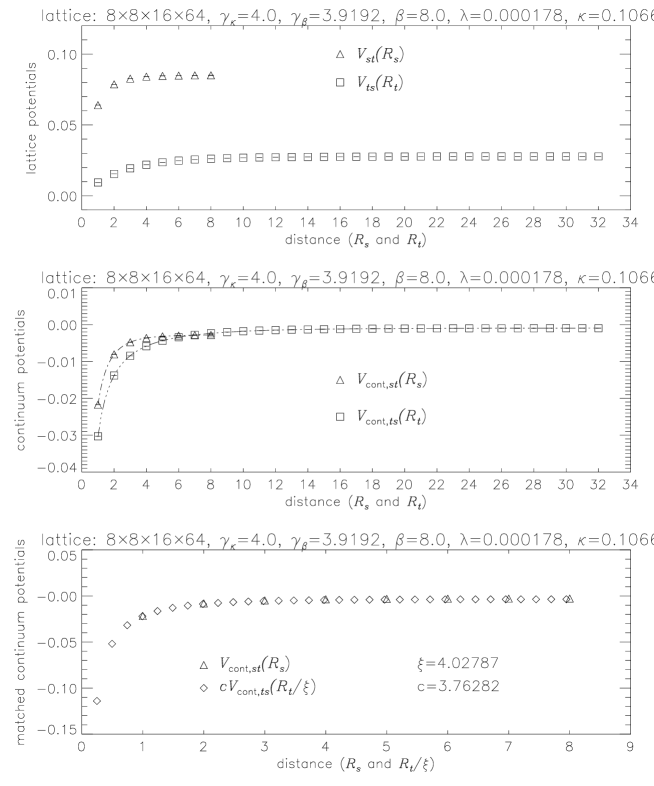
FIG. 6.: Matching of the (subtracted) lattice potentials at the perturbative parameters. The error bars are smaller than the symbols.

D Evaluation of the non-perturbative asymmetries and comparison with the perturbative result

We have determined the lattice spacing anisotropies $\xi_{i}$ from Higgs ($i=H$) and gauge ($i=W$) boson correlation functions and static potentials ($i=V$) at different pairs of coupling anisotropy parameters. Since $\gamma_{\kappa}$ has been held fixed, each $\xi_{i}$ is looked upon as a function of $\gamma_{\beta}$, and the requirement of space-time symmetry restoration suggests the existence of a unique coupling anisotropy $\gamma_{\beta}^{{\mbox{(np)}}}$, where all $\xi_{i}$ possess the same value $\xi^{{\mbox{(np)}}}$. This defines the non-perturbative anisotropy parameters.

Therefore, we linearly interpolate the numbers $\xi_{ij}\equiv\xi_{i}(\gamma_{\beta,j})$ at the three values $\gamma_{\beta,j}$ of eq. (118) within their errors $\Delta\xi_{ij}$ to a matching point $\big{(}\gamma_{\beta}^{{\mbox{(np)}}},\xi^{{\mbox{(np)}}}\big{)}$ by minimizing the sum of squares

$$\chi^{2}=\sum_{i}\sum_{j}\left\{\frac{\xi_{ij}-(\,\xi^{{\mbox{(np)}}}+c_{i}\,[\,\gamma_{\beta,j}-\gamma_{\beta}^{{\mbox{(np)}}}\,]\,)}{\Delta\xi_{ij}}\right\}^{2}$$ (136)

with respect to $c_{i}$ and the common fit parameters $\gamma_{\beta}^{{\mbox{(np)}}}$ and $\xi^{{\mbox{(np)}}}$. We obtain the final results

$$8^{2}\times 12\times 48 \gamma_{\beta}^{{\mbox{(np)}}}=3.911(43)\,,\quad\xi^{{\mbox{(np)}}}=4.040(35)$$ : (137)

$$8^{2}\times 16\times 64 \gamma_{\beta}^{{\mbox{(np)}}}=3.920(19)\,,\quad\xi^{{\mbox{(np)}}}=4.040(26)$$ : (138)

with errors coming from 5000 normally distributed random data. Figure 7 illustrates that both points agree with the simulated $\xi_{i}$ at the perturbative $\gamma_{\beta}$–value as well as with the perturbative point itself, and finite-size effects appear to be remarkably small.

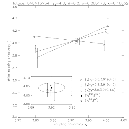
FIG. 7.: Final $\xi$–evaluation for both lattices from the three simulation points, whose equal abscissas are slightly displaced for better visualization. The inserts show the average matching points and its error ellipses, which enclose both the numerical estimates at $\gamma_{\beta}=3.919$ and the perturbative result.

It remains to be mentioned that (138) includes the $\xi_{V}$–values — which incidentally were not available at $\gamma_{\beta}=3.919$ for the smaller lattice — from the matching of the potentials. Using the weighted averages of the two screening mass ratios in table V in place of the former, we get the similar results $\gamma_{\beta}^{{\mbox{(np)}}}=3.921(38)$, $\xi^{{\mbox{(np)}}}=4.038(29)$, and $\gamma_{\beta}^{{\mbox{(np)}}}=3.921(19)$, $\xi^{{\mbox{(np)}}}=4.038(26)$, respectively.

All estimates signal a perfect confirmation of the perturbative results $\gamma_{\beta}^{{\mbox{(p)}}}=3.919$ and $\xi^{{\mbox{(p)}}}=4.052$ calculated in section II. and quoted in item e. at the end of subsection II.B. There is no evidence that the unknown higher-order corrections in $g^{2}$ and $\lambda$ could lead to any visible modifications, which would make the applicability of one-loop perturbation theory to the anisotropy parameters doubtful. In conclusion, the non-perturbative contributions can not be resolved within the intrinsic errors of numerical simulations, and as a consequence, the perturbative choice of the anisotropy parameters in investigations with the SU(2)-Higgs model with asymmetric lattice parameters is justified also for Higgs masses $m_{H}\geq 80$ GeV.

IV Summary

In summary, we have worked out the complete one-loop perturbation theory of the SU(2)-Higgs model on lattices with asymmetric lattice spacings in $R_{\xi}$ gauges. We have determined the critical hopping parameter and the coupling asymmetries in one-loop perturbation theory, as a function of the asymmetry parameter $\xi$. We have proven by explicit calculations the gauge independence of these results in $R_{\xi}$ gauges. We have perturbatively studied the approach to the continuum limit of the finite temperature theory and have determined the optimal choice of $\xi$ ensuring the most economical lattice simulation for a given precision determination of the physical parameters.

To test the relevance of the perturbative results to non-perturbative studies we have determined the non-perturbative coupling anisotropies using lattice simulations. Three channels have been studied, namely Higgs and W–masses as well as the static potential. For our parameters, i.e. Higgs mass near 80 GeV, $g^{2}\approx 0.5$ and $\xi=4$ the perturbative results agree with the non-perturbative determination within the (high) accuracy of the latter. This result opens the possibility to perform lattice simulation using the perturbative coupling anisotropies without the need of a non-perturbative determination. In particular our results are essential to study the electroweak phase transition for Higgs boson masses around or above 80 GeV and determine the properties of the hot electroweak plasma.

This work was partially supported by Hungarian Science Foundation grant under Contract No. OTKA-T016248 and OTKA-T022929 and by Hungarian Ministry of Education grant No. FKFP-0128/1997.

REFERENCES

• [1] V. A. Kuzmin, V. A. Rubakov, M. E. Shaposhnikov, Phys. Lett. B155, 36 (1985).
• [2] P. Arnold, O. Espinosa, Phys. Rev. D47 3546 (1993); W. Buchmüller, Z. Fodor, T. Helbig , D. Walliser, Ann. Phys. 234 260 (1994).
• [3] Z. Fodor , A. Hebecker, Nucl. Phys. B432 127 (1994).
• [4] W. Buchmüller, Z. Fodor, A. Hebecker, Nucl. Phys. B447 317 (1995).
• [5] B. Bunk, E.-M. Ilgenfritz, J. Kripfganz , A. Schiller, Nucl. Phys. B403 453 (1993).
• [6] K. Farakos, K. Kajantie, K. Rummukainen, M. Shaposhnikov, Nucl. Phys. B407 356 (1993); B425 67 (1994); B442 317 (1995); K. Kajantie, M. Laine, K. Rummukainen, M. Shaposhnikov, Nucl.Phys. B466 189 (1996).
• [7] M. Laine, Nucl. Phys. B451 484 (1995).
• [8] F. Karsch, T. Neuhaus , A. Patkós, Nucl. Phys. B441 629 (1995).
• [9] A. Jakovác, K. Kajantie, A. Patkós, Phys. Rev. D49 6810 (1994); A. Jakovác, A. Patkós, P. Petreczky, Phys.Lett. B367 283 (1996).
• [10] H.-G. Dosch, J. Kripfganz, A. Laser, M. G. Schmidt, Phys. Lett. B365 213 (1995); E. M. Ilgenfritz, J. Kripfganz, H. Perlt, A. Schiller, Phys. Lett. B356 561 (1995).
• [11] W. Buchmüller, O. Philipsen, Nucl. Phys. B443 47 (1995); O. Philipsen, M. Teper, H. Wittig, Nucl.Phys. B469 445 (1996).
• [12] F. Csikor, Z. Fodor, J. Hein, K. Jansen, A. Jaster, I. Montvay, Phys. Lett. B334 405 (1994); F. Csikor, Z. Fodor, J. Hein , J. Heitger, Phys. Lett. B357 156 (1995).
• [13] Z. Fodor, J. Hein, K. Jansen, A. Jaster, I. Montvay, Nucl. Phys. B439 147 (1995).
• [14] F. Csikor, Z. Fodor, J. Hein, A. Jaster, I. Montvay, Nucl. Phys. B474 421 (1996).
• [15] Z. Fodor, K. Jansen, Phys. Lett. B331 119 (1994); B. Bunk, Nucl. Phys. B42 (Proc. Suppl.) 566 (1995).
• [16] K. Jansen, Nucl. Phys. B47 (Proc. Suppl.) 196 (1996); K. Rummukainen, Nucl. Phys. B53 (Proc. Suppl.) 30 (1997).
• [17] F. Csikor, Z. Fodor, J. Hein, J. Heitger, A. Jaster, I. Montvay, Nucl. Phys. B53 (Proc. Suppl.) 612 (1997).
• [18] K. Kajantie, M. Laine, K. Rummukainen, M. Shaposhnikov, Phys. Rev. Lett. 77 2887 (1996).
• [19] F. Karsch, T. Neuhaus, A. Patkós, J. Rank, Nucl. Phys. B53 (Proc. Suppl.) 623 (1997); M. Gürtler, E.-M. Ilgenfritz, A. Schiller, Phys. Rev. D56 3888 (1997).
• [20] I. Bender et al., Nucl. Phys. B17 (Proc. Suppl.) 387 (1990); B. Bunk, ibid B42 566 (1995).
• [21] F. Karsch, Nucl. Phys. B205 285 (1982).
• [22] F. Karsch, O. Stamatescu, Phys. Lett. B227 153 (1989).
• [23] F. Csikor, Z. Fodor, Phys. Lett. B380 113 (1996).
• [24] I. Montvay, Phys. Lett. B172 (1986) 71; Nucl. Phys. B293 479 (1987) .
• [25] I. Montvay, G. Münster, Quantum fields on a lattice Cambridge Univ. Press, Cambridge (1994)
• [26] A. Hasenfratz, P. Hasenfratz, Phys. Rev. D34 3160 (1986).
• [27] U. Wolff, Phys. Lett. B288 166 (1992); K. Akemi et al., Phys. Lett. B328 407 (1994).
• [28] J. Hein, J. Heitger, Phys. Lett. B385 242 (1996).
• [29] G. Curci, G. Pafutti, R. Tripiccione, Nucl. Phys. B240 [FS12] 91 (1984).
• [30] U. Heller, F. Karsch, Nucl. Phys. B251 [FS13] 254 (1985).
• [31] W. Langguth, I. Montvay, P. Weisz, Nucl. Phys. B277 11 (1986).
• [32] R. Sommer, Nucl. Phys. B411 839 (1994).
• [33] C. Michael, Phys. Rev. D49 2616 (1994); C. Michael, A. McKerrel, Phys. Rev. D51 3745 (1995).
• [34] G. Burgers, F. Karsch, A. Nakamura, I.O. Stamatescu, Nucl. Phys. B304 587 (1988).