ITEP-TH-16/98
MPI/PhT/98-24
March 1998

1 Introduction

The abelian Higgs model in $3+1$ dimensions possesses the vortex topological defects called Abrikosov–Nielsen–Olesen (ANO) strings [1]. These strings carry quantized magnetic flux and therefore they interact with the charged particles through the analog [2] of the Aharonov–Bohm (AB) effect [3]. The AB effect has the topological origin: the corresponding interaction is proportional to the linking number of the string world sheet and the particle world trajectories. Due to AB interaction of the ANO strings and charged particles the ANO strings may induce a long–range interaction between the particles [4]. To study the role of the AB effect in the particle–anti-particle potential we calculate numerically in lattice Abelian Higgs model the correlations of the Wilson loop on the contour ${\cal C}$ and the linking number of the ANO strings with this contour. We find that in the vicinity of the Coulomb–Higgs phase transition the AB interaction provides the dominant contribution to the Wilson loop.

Another aim of the paper is to study the fractal properties of the ANO strings. We measure the fractal dimensionality $D_{f}$ of the ANO strings and we find that $D_{f}$ is close to 2 in the Higgs phase and it is much larger in the Coulomb phase. This fact is in agreement with the observation [5] that the vortex strings are condensed in the Coulomb phase and they are dilute in the Higgs phase.

In Section 2 we show the ANO strings representation for the partition function of the $4D$ abelian Higgs model with the Villain action and we show how the AB effect emerges in the path–integral formalism. Section 3 is devoted to the discussion on the fractal properties of the ANO strings and the role of the AB effect in the inter–particle potential. Two quantities $R$ and ${\cal C}$ which characterize the contribution of the AB interaction to the inter–particle potentials are suggested. These quantities and the fractal dimension of the ANO strings are calculated numerically and the results are presented in Section 4.

2 Abrikosov–Nielsen–Olesen Strings and Aharonov–Bohm Effect on the Lattice

The partition function of $4D$ non–compact abelian Higgs model on the lattice is:

$${\cal Z}=\int\limits_{-\infty}^{+\infty}{{\cal D}}A\int\limits_{-\pi}^{+\pi}{{\cal D}}\varphi\sum_{l(\mbox{\scriptsize c}_{\mbox{$\scriptstyle 1$}})\in{Z\!\!\!Z}}\exp\left\{-\beta\|{\rm d}A\|^{2}-\gamma\|{\rm d}\varphi+2\pi l+A\|^{2}\right\}\,,\\$$ (1)

where $A$ is the non–compact gauge field, $\varphi$ is the phase of the Higgs field and $l$ is the integer–valued one–form. For simplicity we consider the limit of the infinite Higgs boson mass (the radial part of the Higgs field is frozen) and we use the Villain form of the action.

One can rewrite [6] integral (1) as the sum over the closed string trajectories using the analogue of Berezinski–Kosterlitz–Thauless (BKT) transformation [8]:

$${\cal Z}\propto{\cal Z}^{BKT}=const.\,\sum_{\stackrel{{\scriptstyle\scriptstyle\mbox{}^{\ast}\sigma(\mbox{}^{\ast}\mbox{\scriptsize c}_{\mbox{$\scriptstyle 2$}})\in{Z\!\!\!Z}}}{{\delta\mbox{}^{\ast}\sigma=0}}}\exp\left\{-4\pi^{2}\gamma\left(\mbox{}^{\ast}\sigma,{(\Delta+m^{2})}^{-1}\mbox{}^{\ast}\sigma\right)\right\}\,,$$ (2)

where $m^{2}=\gamma/\beta$ is the classical mass of the vector boson $A$. Closed surfaces $\mbox{}^{\ast}\sigma$ on the dual lattice represent the string world sheets. It can be easily seen from eq.(2) that the surfaces $\mbox{}^{\ast}\sigma$ interact with each other through the Yukawa forces.

Consider the quantum average of the Wilson loop $W_{1\over N}({\cal C})=\exp\Bigl{\{}i\frac{1}{N}(A,j_{\cal C})\Bigr{\}}$ for the particle with the charge $1/N$. Using the BKT transformation we get the following formula [6, 9]:

$${<W_{1\over N}({\cal C})>}=\frac{1}{{\cal Z}^{BKT}}\sum_{\stackrel{{\scriptstyle\scriptstyle\mbox{}^{\ast}\sigma(\mbox{}^{\ast}\mbox{\scriptsize c}_{\mbox{$\scriptstyle 2$}})\in{Z\!\!\!Z}}}{{\delta\mbox{}^{\ast}\sigma=0}}}\exp\biggl{\{}-4\pi^{2}\gamma\left(\mbox{}^{\ast}\sigma,{\left(\Delta+m^{2}\right)}^{-1}\mbox{}^{\ast}\sigma\right)$$

$$-\frac{1}{4\beta N^{2}}(j_{\cal C},(\Delta+m^{2})^{-1}j_{\cal C})+2\pi i\frac{1}{N}\left(\mbox{}^{\ast}j_{\cal C},{\left(\Delta+m^{2}\right)}^{-1}{\rm d}\mbox{}^{\ast}\sigma\right)-2\pi i\frac{1}{N}{I\!\!L}\left(\mbox{}^{\ast}\sigma,j_{\cal C}\right)\biggr{\}}\,.$$ (3)

The first three terms in this expression are the short–range Yukawa forces between defects and particles. The last long–range term has the topological origin: ${I\!\!L}(\mbox{}^{\ast}\sigma,j_{\cal C})$ is the linking number between the world trajectories of the string world sheets $\mbox{}^{\ast}\sigma$ and the contour which define the Wilson loop, $j_{\cal C}$:

$${I\!\!L}(\mbox{}^{\ast}\sigma,j_{\cal C})=(\mbox{}^{\ast}j_{\cal C},{\Delta}^{-1}{\rm d}\mbox{}^{\ast}\sigma)=(\mbox{}^{\ast}j_{\cal C},\mbox{}^{\ast}v)\,;\,\,\mbox{}^{\ast}\sigma=\delta\mbox{}^{\ast}v\,.$$ (4)

In four dimensions the trajectory of the string $\mbox{}^{\ast}\sigma$ is a closed surface and the linking number ${I\!\!L}$ is equal to the number of points at which the loop $j_{\cal C}$ intersects the three dimensional volume $\mbox{}^{\ast}v$ bounded by the surface $\mbox{}^{\ast}\sigma$. The equation (4) is the lattice analogue of the 4D Gauss formula for the linking number. The strings can be considered as the solenoids with magnetic flux which scatter the electrically charged particles. After the scattering the wave–function of the charged particle acquire an additional phase which is observable. This shift in phase is the AB effect in the field theory [2, 6, 9].

3 Fractal Dimension of Strings and Parameters of Topological Interaction

The abelian Higgs model with non-compact gauge field has Coulomb and Higgs phases. The strings are dilute in the Higgs phase and they are condensed in the Coulomb phase [5]. The condensed phase of the ANO strings is characterized by large string clusters. One of the characteristics of the string network is the fractal dimensionality $D_{f}$ which is defined as follows. Let us denote the number of the plaquettes (links) of the string world–sheet as $B$ (L). Each plaquette $P$ contributes the value $|\mbox{}^{\ast}\sigma_{P}|$ to the quantity $B$ and each link $l$ contributes to the quantity $L$ the value $\max_{P\ni l}|\mbox{}^{\ast}\sigma_{P}|$ if the link $l$ belongs to the string world sheets or zero otherwise. We define the fractal dimension as

$$D_{f}=1+2B/L\,.$$ (5)

One can check, that if the closed string has no selfintersections, then $D_{f}=2$. If the string form 3– or 4– dimensional clusters, then $D_{f}$ equals to $3$ or $4$, respectively. We expect, that if the strings are not condensed, then $D_{f}$ is close to $2$ since the number of the self–intersections is small. If the strings are condensed, then $D_{f}>2$.

In the previous Section the topological (AB) interaction of the ANO strings with the fractionally charged particles was shown. This interaction is proportional to the linking number of the particle trajectory and the string world sheet. One of the parameters which can show the role of the AB effect in the quantum averages of the Wilson loops is the following. The contribution of the given field configuration to the Wilson loop on the contour ${\cal C}$ is $\cos\Bigl{(}\frac{1}{N}(A,j_{\cal C})\Bigr{)}$, while the contribution to this Wilson loop from the AB effect extracted from the same configuration is: $\cos\Bigl{(}\frac{2\pi}{N}{I\!\!L}(\mbox{}^{\ast}\sigma,j_{\cal C})\Bigr{)}$. The quantitative parameter which measures the correlation between these two contributions is:

$$C({\cal C},N) = <\cos\Bigl{(}\frac{1}{N}(A,j_{\cal C})\Bigr{)}\cos\Bigl{(}\frac{2\pi}{N}{I\!\!L}(\mbox{}^{\ast}\sigma,j_{\cal C})\Bigr{)}>-$$ (6)

$$<\cos\Bigl{(}\frac{1}{N}(A,j_{\cal C})\Bigr{)}>\,<\cos\Bigl{(}\frac{2\pi}{N}{I\!\!L}(\mbox{}^{\ast}\sigma,j_{\cal C})\Bigr{)}>\,.$$

If correlator (6) is not zero then the AB effect contributes into the quantum average of the Wilson loop. Then another question appears: can this topological interaction provide a dominant contribution to the Wilson loop? To check that we study in the next Section the difference between the Wilson loop average and the average of the AB contribution to the Wilson loop:

$$R=<\cos\Bigl{(}\frac{1}{N}(A,j_{\cal C})\Bigr{)}>-<\cos\Bigl{(}\frac{2\pi}{N}{I\!\!L}(\mbox{}^{\ast}\sigma,j_{\cal C})\Bigr{)}>\,.$$ (7)

4 Numerical Results

In numerical calculations we study the abelian Higgs model with the Wilson type of the action in the London limit:

$$S=\beta{||{\rm d}A||}^{2}-\gamma\sum_{l\in links}\cos{({\rm d}\phi+A)}_{l}\,.$$

The ANO strings are extracted from the field configurations as follows [10, 5]:

$$\mbox{}^{\ast}\sigma=\mbox{}^{\ast}{\rm d}n\,,\quad({\rm d}\varphi+A+2\pi n)\in(-\pi,\pi]\,,\quad n\in{Z\!\!\!Z}\,.$$

The calculations has been performed on $16^{4}$ lattice in the gauge ${\rm d}\phi=0$. For each value of the parameters $(\beta,\gamma)$ 50-100 statistically independent configurations have been generated by the usual Monte-Carlo method. The dependence of the fractal dimension $D_{f}$ (5) on the parameters $\beta$ and $\gamma$ is shown on Figure 1(a). The fractal dimension of the ANO strings is close to $2$ in the Higgs phase and it is larger in the Coulomb phase. Thus the string network in the Coulomb phase consists of the clusters with the large number of selfintersections. The transition from the dense string phase to the phase of the dilute strings is rather sharp, see Figure 1(b).

Figure 2 shows the correlator $C$ (6) for $4\times 4$ Wilson loop and for the charge $Q=1/10$ ($W({\cal C})=\exp\{iQ(A,j_{\cal C}\}$). Since $C>0$ then the topological interaction contributes to the test particle interaction.

In Figure 3 (a,b) the quantity $R$ defined by eq.(7) is shown. We calculated $R$ for various contours ${\cal C}$ ($3\times 3$, $3\times 4$, $4\times 4$, $4\times 5$, $5\times 5$) and for various charges of the test particle ($Q=1/2,1/3,1/4,1/10$). It is interesting that the zeroes of $R$ lie in the vicinity of the line of the phase transition. The positions of the zeroes depends very slightly on the charge $N$ and on the shape of the Wilson loop. The parameter $R$ is negative in the Higgs phase and is positive in the Coulomb phase. Thus near the phase transition the expectation value of the Wilson loop is due to the topological (AB) interaction.

We conclude that the Abrikosov–Nielsen–Olesen strings in $4D$ Abelian Higgs model form a fractal cluster in the Coulomb phase ($D_{f}>2$); in the Higgs phase $D_{f}\sim 2$, thus in this phase in the string model (2) the strings are not crumpled. The Aharonov–Bohm interaction of the strings with charged particles gives the dominant contribution to the Wilson loop quantum average for non–integer test charges in the vicinity of the Coulomb–Higgs phase transition. Thus in this region the Abelian Higgs model behaves as a topological theory, we study the origin of this fact in the subsequent publications.

Figures

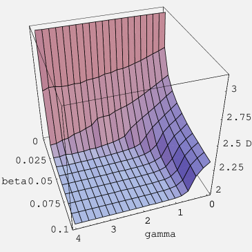
(a)	(b)

Figure 1: (a)The fractal dimension of the ANO strings, $D_{f}$, versus $\beta$ and $\gamma$. (b) The fractal dimension $D_{f}$, versus $\gamma$ at $\beta=0.1$; the phase transition from Coulomb phase ($\gamma<\gamma_{c}$) to Higgs phase ($\gamma>\gamma_{c}$) is at $\gamma=\gamma_{c}\approx 0.48$.

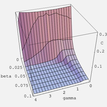
Figure 2: The correlator $C$ (6) for $4\times 4$ Wilson loop, $Q=1/10$.

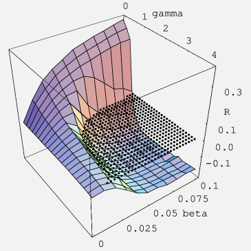
(a)	(b)

Figure 3: (a) The quantity $R$ (7) for $4\times 4$ Wilson loop, $Q=1/10$. The plane $R=0$ is shown by dots. (b) The dependence of the quantity $R$ on $\gamma$ at $\beta=0.1$; the phase transition from Coulomb phase ($\gamma<\gamma_{c}$) to Higgs phase ($\gamma>\gamma_{c}$) is at $\gamma=\gamma_{c}\approx 0.48$.

References

-
[1]
A.A. Abrikosov, Sov. Phys. JETP, 32 (1957) 1442;
H.B. Nielsen and P. Olesen, Nucl. Phys., B61 (1973) 45. - [2] M.G. Alford and F. Wilczek, Phys. Rev. Lett., 62 (1989) 1071; L.M. Kraus and F. Wilczek, Phys. Rev. Lett., 62 (1989) 1221; M.G. Alford, J. March–Russel and F. Wilczek, Nucl. Phys., B337 (1990) 695; J. Preskill and L.M. Krauss, Nucl. Phys., B341 (1990) 50; E.T. Akhmedov et.al., Phys.Rev. D53 2097 (1996).
- [3] Y. Aharonov and D. Bohm, Phys.Rev. 115 (1959) 485.
- [4] F.A. Bais, A. Morozov, M. de Wild Propitius, Phys. Rev. Lett. 71 (1993) 2383; M.N. Chernodub, F.V. Gubarev and M.I. Polikarpov, JETP Lett, 63 (1996) 516, hep-lat/9607045; Phys. Lett.B416 (1998) 379; Nucl.Phys.Proc.Suppl. 53 (1997) 581; hep-lat/9607045.
- [5] M. Chavel, Phys. Lett. B378 (1996) 227.
- [6] M.I. Polikarpov, U.-J. Wiese and M.A. Zubkov Phys. Lett., B 309 (1993) 133.
- [7] P. Becher and H. Joos, Z. Phys., C15 (1982) 343.
- [8] V.L. Beresinskii, Sov. Phys. JETP, 32 (1970) 493; J.M. Kosterlitz and D.J. Thouless, J. Phys., C6 (1973) 1181.
- [9] M.N. Chernodub and M.I. Polikarpov, Proceedings of the International Workshop on Nonperturbative Approaches to QCD, Trento, Italy, 10-29 Jul 1995, hep-th/9510014.
- [10] J. Ranft, J. Kripfganz and G. Ranft, Phys.Rev. D28 (1983) 360.
- [11] A.K. Bukenov et.al., Phys. At. Nucl. 56 (1993) 122 (Yad. Fiz. 56 (1993) 214).