Corrections to Finite-Size Scaling in the Lattice $N$-Vector Model for $N=\infty$

Abstract

We compute the corrections to finite-size scaling for the $N$-vector model on the square lattice in the large-$N$ limit. We find that corrections behave as $\log L/L^{2}$. For tree-level improved hamiltonians corrections behave as $1/L^{2}$. In general $l$-loop improvement is expected to reduce this behaviour to $1/(L^{2}\log^{l}L)$. We show that the finite-size-scaling and the perturbative limit do not commute in the calculation of the corrections to finite-size scaling. We present a detailed study of the corrections for the $RP^{\infty}$-model.

1 Introduction

In the study of statistical models it is extremely important to understand finite-size corrections. Indeed in experiments and in numerical work it is essential to take into account the finite size of the system in order to extract correct infinite-volume predictions from the data. Finite-size scaling (FSS) [1, 2, 3, 4, 5] concerns the critical behaviour of systems in which one or more directions are finite, even though microscopically large, and it is therefore essential in the analysis of experimental data in many situations, for instance, for films of finite thickness. Numerically FSS can be used in a variety of ways to extract informations on infinite-volume systems. A very interesting method to extract critical indices comparing data on lattices of different sizes was introduced by Nightingale [6], the so-called phenomenological renormalization group. Recently FSS has been used to obtain precise predictions at very large values of the correlation length from simulations on small lattices. This extrapolation technique was introduced by Lüscher, Weisz and Wolff [7] and subsequently applied to many different models [8, 9, 10, 11, 12, 13]: a careful theoretical analysis (see Sect. 5.1.2 of Ref. [13]) shows that the method is extremely convenient for asymptotically free theories and indeed one was able to simulate the O(3) $\sigma$-model [10] up to $\xi\approx 10^{5}$ and the $SU(3)$ chiral model [12, 13] up to $\xi\approx 4\cdot 10^{5}$ using relatively small lattices ($L\leq 512$). In order to use these techniques reliably it is extremely important to have some theoretical prediction on the behaviour of the corrections to FSS. One can use this information in two different ways. A possibility is to take advantage of the theoretical prediction to extrapolate the Monte Carlo data to the FSS limit — that still involves a limit $L\to\infty$ — in the spirit of Ref. [7]. One also needs this information if one determines the FSS curve by comparing data from simulations on lattices of different sizes as proposed in Ref. [9]. For instance checking the absence (within error bars) of corrections to FSS for lattices of sizes $64\leq L\leq 256$ is enough if the corrections vanish as $1/L^{2}$ while it can be totally misleading if corrections behaving as $1/\log L$ are present (this is the case for instance of the four-state Potts model, see Ref. [14]).

A second topic that will be extensively discussed in this paper is the improvement of lattice hamiltonians [15, 16, 17, 18, 19]. The idea behind all these attempts is to modify the lattice hamiltonian with the addition of irrelevant operators in order to reduce lattice artifacts: in this way one hopes to have scaling and FSS at shorter correlation lengths. For general statistical models this is a non-trivial program. For asymptotically-free theories the idea is much simpler to implement since in this case improvement can be discussed using perturbation theory.

In this paper we will study the problem of corrections to FSS and improvement in the context of the large-$N$ $N$-vector model. This theory provides the simplest example for the realization of a nonabelian global symmetry. Its two-dimensional version has been extensively studied because it shares with four-dimensional gauge theories the property of being asymptotically free in the weak-coupling perturbative expansion [20, 21, 22]. This picture predicts a nonperturbative generation of a mass gap that controls the exponential decay at large distance of the correlation functions.

Besides perturbation theory, the two-dimensional $N$-vector model can be studied using different techniques. It can be solved in the $N=\infty$ limit [23, 24] and $1/N$ corrections can be systematically calculated [25, 26, 27]. An exact $S$-matrix can be computed [28, 29] and, using the thermodynamic Bethe ansatz, the exact mass-gap of the theory in the limit $\beta\to\infty$ has been obtained [30, 31]. The model has also been the object of extensive numerical work [32, 33, 10, 34, 35] mainly devoted to checking the correctness of the perturbative predictions [36, 37, 38].

In the large-$N$ limit FSS can be studied analytically [39, 40, 41]. Here we will concentrate on the corrections to FSS in two dimensions and we will compute the deviations from FSS for generic lattice interactions. We will show that in general corrections to FSS behave as $\log L/L^{2}$. This is in agreement with a general renormalization-group argument that shows that corrections to FSS are controlled by the first subleading operator [42]. Tree-level improvement changes the behaviour by a logarithm of $L$: these actions have corrections behaving as $1/L^{2}$. Subsequent improvement should reduce the corrections to $1/(L^{2}\log L)$ and so on. Full $O(a^{2})$ improvement to all orders of perturbation theory provides an action with corrections behaving as $\log L/L^{4}$.

Besides the standard $N$-vector model we will also discuss a mixed $N$-vector/$RP^{N-1}$-model [24, 43]. There are two reasons why we decided to include this computation: first of all, for large values of $N$, models with only two-spin interactions show many simplifying features: for instance in the $\beta$-function only the leading term does not vanish. For this reason one may expect that the behaviour of the corrections for this class of models is far simpler than in generic models. Instead the mixed $N$-vector/$RP^{N-1}$-model shows a more complex behaviour and, for instance, the $\beta$-function is non trivial to all orders of perturbation theory. We find that in the mixed model the corrections behave as $(\log L/L^{2})f(L)$ where $f(L)$ is a non-trivial function such that $f(\infty)$ is finite and that admits an asymptotic expansion in powers of $1/\log L$. The presence of powers $1/(L^{2}\log^{n}L)$ is somewhat unexpected from the point of view of perturbation theory. We will show that this is related to the non commutativity of the limits $L\to\infty$ and $\beta\to\infty$. In other words the perturbative limit $\beta\to\infty$ at $L$ fixed followed by the limit $L\to\infty$ gives results that are different from the FSS limit. The commutativity of these two limits has been the object of an intense debate. The standard wisdom is that the two limits are identical, but this point has been seriously questioned by Patrascioiu and Seiler [44] (for an answer to these criticisms see Ref. [45]) together with many other assumptions derived from perturbation theory [46]. Our calculation shows that, if the standard assumption is true, it is a result far from obvious: indeed the limits are different for the corrections to FSS.

A second motivation lies in recent work [47, 48] on the $RP^{N-1}$ models that has shown the possibility that these models have very large FSS corrections. We wanted to understand if there is any sign of this phenomenon in the large-$N$ limit. Our explicit calculation shows that $RP^{\infty}$ has corrections that are larger than those of the $N$-vector model. Depending on the observable, for reasonable lattice sizes, we find an increase by a factor of 6-15. This is in qualitative agreement with the scenario of Ref. [47].

The paper is organized as follows: in Sect. 2 we define the models we consider, and compute various observables in the large-$N$ limit. In Sect. 3 we discuss the corrections to FSS for the $N$-vector model and in Sect. 4 we extend our results to the mixed $N$-vector/$RP^{N-1}$ model. In Sect. 5 we present our conclusions.

In the Appendices we report some general results on the FSS behaviour of lattice sums. These results are of general interest and may be applied in many other contexts: in particular they may be used to study FSS properties of models that have a height (SOS) representation (see Refs. [49, 50] and references therein). In Appendix A we define a set of basic functions that appear in all our results and we report some of their properties. We extend here the results of Ref. [51]. In Appendix B we give an algorithmic procedure that allows to compute the expansion in powers of $1/L^{2}$ of any sum involving powers of the lattice propagator for a Gaussian model with arbitrary interaction in the FSS limit. As an example we report the explicit formulae that are needed in our main discussion. In Appendix C we report the asymptotic behaviour of some lattice integrals.

Preliminary results of this work were presented at the Lattice ’96 Conference [52].

2 The models

In this paper we will study the finite-size-scaling properties of the classical $N$-vector model on a square lattice with local, translation- and parity-invariant ferromagnetic interactions. The hamiltonian is given by

$${\cal H}=\,N\sum_{x,y}J(x-y)\mbox{\boldmath$\sigma$}_{x}\cdot\mbox{\boldmath$\sigma$}_{y}\;,$$ (2.1)

where the fields $\mbox{\boldmath$\sigma$}_{x}$ satisfy $\mbox{\boldmath$\sigma$}_{x}^{2}=1$. The partition function is simply

$$Z=\,\int\prod_{x}d\mbox{\boldmath$\sigma$}_{x}\,e^{-\beta{\cal H}}.$$ (2.2)

We will consider general local interactions. If $\widehat{J}(p)$ is the Fourier transform of $J(x)$, locality and parity invariance imply that $\widehat{J}(p)$ is a continuous function of $p$, even under $p\to-p$. We will require invariance under rotations of $\pi/2$, that is we will assume $\widehat{J}(p)$ symmetric under interchange of ${p}_{1}$ and ${p}_{2}$. Redefining $\beta$ we can normalize the couplings so that

$$\widehat{J}(q)=\widehat{J}(0)-{q^{2}\over 2}+O(q^{4})$$ (2.3)

for $q\to 0$. We also introduce the function

$$w(q)=-2(\widehat{J}(q)-\widehat{J}(0)),$$ (2.4)

that behaves as $q^{2}$ for $q\to 0$. Finally we will require the theory to have the usual (formal) continuum limit: we will assume that the equation $w(q)=0$ has only one solution for $-\pi\leq q_{i}\leq\pi$, namely $q=0$. We will need the small-$q$ behaviour of $w(q)$: we will assume in this limit the form

$$w(q)=\,\hat{q}^{2}+\alpha_{1}\,\sum_{\mu}\hat{q}^{4}_{\mu}+\alpha_{2}\ (\hat{q}^{2})^{2}+O(q^{6}),$$ (2.5)

where $\alpha_{1}$ and $\alpha_{2}$ are arbitrary constants. Here $\hat{q}^{2}=\hat{q}^{2}_{1}+\hat{q}^{2}_{2}$, $\hat{q}=2\sin(q/2)$.

Let us give some examples we will use in the following. The standard $N$-vector model with hamiltonian

$$H^{std}\,=\,-N\sum_{x\mu}\mbox{\boldmath$\sigma$}_{x}\cdot\mbox{\boldmath$\sigma$}_{x+\mu}$$ (2.6)

corresponds to $w(q)=\hat{q}^{2}$ and thus we have $\alpha_{1}=\alpha_{2}=0$. Other possibilities are:

1. the Symanzik improved hamiltonian [15]

   $$H^{Sym}=-N\sum_{x\mu}\left({4\over 3}\mbox{\boldmath$\sigma$}_{x}\cdot\mbox{\boldmath$\sigma$}_{x+\mu}\,-\,{1\over 12}\mbox{\boldmath$\sigma$}_{x}\cdot\mbox{\boldmath$\sigma$}_{x+2\mu}\right),$$ (2.7)

   for which we have

   $$w(q)=\hat{q}^{2}+{1\over 12}\sum_{\mu}\hat{q}^{4}_{\mu},$$ (2.8)

   and $\alpha_{1}=1/12$ and $\alpha_{2}=0$;

2. the “diagonal” hamiltonian [53]

   $$H^{diag}=-N\sum_{x}\left({2\over 3}\sum_{\mu}\mbox{\boldmath$\sigma$}_{x}\cdot\mbox{\boldmath$\sigma$}_{x+\mu}\,+\,{1\over 6}\sum_{\hat{d}}\mbox{\boldmath$\sigma$}_{x}\cdot\mbox{\boldmath$\sigma$}_{x+\hat{d}}\right)$$ (2.9)

   where $\hat{d}$ are the two diagonal vectors $(1,\pm 1)$, for which we have

   $$w(q)=\,\hat{q}^{2}-{1\over 6}\hat{q}^{2}_{1}\hat{q}_{2}^{2},$$ (2.10)

   and $\alpha_{1}=1/12$ and $\alpha_{2}=-1/12$;

3. the perfect laplacian introduced in various works on the renormalization group [54] and recently revived in connection with the perfect actions [17]:

   $${1\over w(q)}\,=\,{1\over 3\kappa}+\sum_{l_{1}=-\infty}^{\infty}\sum_{l_{2}=-\infty}^{\infty}{1\over(q_{1}+2\pi l_{1})^{2}+(q_{2}+2\pi l_{2})^{2}}\,{\hat{q}_{1}^{2}\hat{q}_{2}^{2}\over(q_{1}+2\pi l_{1})^{2}(q_{2}+2\pi l_{2})^{2}}$$ (2.11)

   for which $\alpha_{1}=1/12$ and $\alpha_{2}=(\kappa-4)/(12\kappa)$.

In general we will speak of tree-level improved hamiltonians whenever $\alpha_{1}=1/12$, $\alpha_{2}=0$: in this case, for $q^{2}\to 0$,

$$w(q)=q^{2}+O(q^{6}).$$ (2.13)

The hamiltonians (2.7) and (2.11) for $\kappa=4$ are examples of tree-level improved hamiltonians.

In order to study the finite-size-scaling properties we must specify the geometry. We will consider here a square lattice of size $L\times T$ or a strip of width $L$ with periodic boundary conditions in the finite direction(s). The large-$N$ limit of this model is well known [23]. The theory is parametrized by a mass parameter $m^{2}_{L,T}$ related to $\beta$ by the gap equation

$$\beta={1\over LT}\sum_{n_{1},n_{2}}{1\over w(p)+m^{2}_{L,T}}\,\equiv{\cal I}_{L,T}(m^{2}_{L,T}),$$ (2.14)

where $p_{1}=2\pi n_{1}/L$, $p_{2}=2\pi n_{2}/T$ and the sum extends over $0\leq n_{1}\leq L-1$ and $0\leq n_{2}\leq T-1$. The two-point isovector Green’s function is then given by

$$G_{V}(x-y;L,T)\equiv\langle\mbox{\boldmath$\sigma$}_{x}\cdot\mbox{\boldmath$\sigma$}_{y}\rangle={1\over\beta}\,{1\over LT}\sum_{n_{1},n_{2}}{e^{ip\cdot(x-y)}\over w(p)+m^{2}_{L,T}}.$$ (2.15)

All other Green’s functions are obtained from $G_{V}(x;L,T)$ using the factorization theorem

$$\langle(\mbox{\boldmath$\sigma$}_{x_{1}}\cdot\mbox{\boldmath$\sigma$}_{y_{1}})(\mbox{\boldmath$\sigma$}_{x_{2}}\cdot\mbox{\boldmath$\sigma$}_{y_{2}})\ldots(\mbox{\boldmath$\sigma$}_{x_{n}}\cdot\mbox{\boldmath$\sigma$}_{y_{n}})\rangle\,=\,\langle(\mbox{\boldmath$\sigma$}_{x_{1}}\cdot\mbox{\boldmath$\sigma$}_{y_{1}})\rangle\langle(\mbox{\boldmath$\sigma$}_{x_{2}}\cdot\mbox{\boldmath$\sigma$}_{y_{2}})\rangle\ldots\langle(\mbox{\boldmath$\sigma$}_{x_{n}}\cdot\mbox{\boldmath$\sigma$}_{y_{n}})\rangle.$$ (2.16)

In particular we will consider the isotensor (spin-two) two-point function

$$G_{T}(x-y;L,T)\equiv\,\langle(\mbox{\boldmath$\sigma$}_{x}\cdot\mbox{\boldmath$\sigma$}_{y})^{2}\rangle-{1\over N}\,=\,\langle\mbox{\boldmath$\sigma$}_{x}\cdot\mbox{\boldmath$\sigma$}_{y}\rangle^{2}+O(1/N).$$ (2.17)

Beside the standard $N$-vector model we will also discuss a mixed $N$-vector/$RP^{N-1}$-model [24, 43, 57, 58]. We will restrict our attention to nearest-neighbour interactions since only in this case the model is easily solvable in the large-$N$ limit. The hamiltonian is given by

$$H^{mix}=-N\,\sum_{\langle xy\rangle}\left[(1-r)\mbox{\boldmath$\sigma$}_{x}\cdot\mbox{\boldmath$\sigma$}_{y}+{r\over 2}(\mbox{\boldmath$\sigma$}_{x}\cdot\mbox{\boldmath$\sigma$}_{y})^{2}\right],$$ (2.18)

where the sum is extended over all links $\langle xy\rangle$ and $r$ is a free parameter varying between 0 and 1. For $r=0$ we have the nearest-neighbour $N$-vector model, while $r=1$ corresponds to the $RP^{N-1}$-model. Notice that for $r=1$ the theory is invariant under local transformations $\mbox{\boldmath$\sigma$}_{x}\to\epsilon_{x}\mbox{\boldmath$\sigma$}_{x}$, $\epsilon_{x}=\pm 1$. Therefore for $RP^{N-1}$ only isotensor observables are relevant. The limit we consider here corresponds to $N\to\infty$ with $r$ fixed. We mention that this is not the only case in which the model is solvable: a different large-$N$ limit is considered in Ref. [58].

Also in this case the theory is parametrized by a mass parameter $m^{2}_{L,T}$ related to $\beta$ by [43]

$$\beta=\,{4I_{L,T}(m_{L,T}^{2})^{2}\over 4I_{L,T}(m_{L,T}^{2})+r(m^{2}_{L,T}I_{L,T}(m^{2}_{L,T})-1)}\;,$$ (2.19)

where

$$I_{L,T}(m_{L,T}^{2})\equiv\,{1\over LT}\sum_{n_{1},n_{2}}{1\over\hat{p}^{2}+m^{2}_{L,T}}\;,$$ (2.20)

with $p_{1}=2n_{1}\pi/L$, $p_{2}=2n_{2}\pi/T$.

The isovector Green’s function is given by

$$G_{V}(x-y;L,T)={1\over{I}_{L,T}(m^{2}_{L,T})}\,{1\over LT}\sum_{n_{1},n_{2}}{e^{ip\cdot(x-y)}\over\hat{p}^{2}+m^{2}_{L,T}}\;.$$ (2.21)

All other correlations are obtained using Eq. (2.16). In the $N$-vector case we can use the gap equation to substitute ${I}_{L,T}(m^{2}_{L,T})$ with $\beta$.

In this paper we will study the finite-size-scaling properties of various quantities. We define the vector and tensor susceptibilities

$$\chi_{V}(L,T) = \sum_{x}G_{V}(x;L,T),$$ (2.22)

$$\chi_{T}(L,T) = \sum_{x}G_{T}(x;L,T).$$ (2.23)

Using the explicit expressions for the two-point functions we get

$$\chi_{V}(L,T) = {1\over{\cal I}_{L,T}(m^{2}_{L,T})m^{2}_{L,T}}$$ (2.24)

$$\chi_{T}(L,T) = {1\over({\cal I}_{L,T}(m^{2}_{L,T}))^{2}}\,{1\over LT}\sum_{n_{1},n_{2}}{1\over(w(p)+m^{2}_{L,T})^{2}}.$$ (2.25)

We want also to define a quantity behaving as a correlation length. In an infinite lattice there are essentially two possibilities. One can define the exponential correlation length from the large-$x$ behaviour of a given two-point function $G(x;\infty)$: one considers a wall-wall correlation function

$$G^{(w)}(y;\infty)=\sum_{x}G((x,y);\infty),$$ (2.26)

and then defines

$$\xi^{(exp)}(\infty)=\,-\lim_{y\to+\infty}{y\over\log G^{(w)}(y;\infty)}\;.$$ (2.27)

The mass gap $\mu(\infty)$ is the inverse of $\xi^{(exp)}(\infty)$. A second possibility is the second-moment correlation length $\xi^{(m)}(\infty)$ that is defined by

$$\left[\xi^{(m)}(\infty)\right]^{2}={1\over 4}{\sum_{x}|x|^{2}G(x;\infty)\over\sum_{x}G(x;\infty)}\;.$$ (2.28)

The factor $1/4$ has been introduced in order to have $\xi^{(m)}(\infty)=\xi^{(exp)}(\infty)$ for Gaussian models.

We must now give the definitions in finite volume. Of course the exponential correlation can only be defined in a strip. In this case we can still use the definition (2.27). For the second-moment correlation length we can use any definition that becomes equivalent to (2.28) in the limit $L,T\to\infty$. We will consider here three different definitions: given a two-point function $G(x;L,T)$ and its Fourier transform $\hat{G}(p;L,T)$ we define

$$\left(\xi^{(m,1)}(L,T)\right)^{2} = {1\over 2\hat{p}_{0x}^{2}}\left[{\hat{G}(0;L,T)\over\hat{G}(p_{0x};L,T)}-1\right]+\,{1\over 2\hat{p}_{0y}^{2}}\left[{\hat{G}(0;L,T)\over\hat{G}(p_{0y};L,T)}-1\right]\;,$$ (2.29)

$$\left(\xi^{(m,2)}(L,T)\right)^{2} = {L^{2}\over 8\pi^{2}}\left(1-{\hat{G}(p_{0x};L,T)\over\hat{G}(0;L,T)}\right)+{T^{2}\over 8\pi^{2}}\left(1-{\hat{G}(p_{0y};L,T)\over\hat{G}(0;L,T)}\right)\;,$$ (2.30)

$$\left(\xi^{(m,3)}(L,T)\right)^{2} = {1\over 4\hat{G}(0;L,T)}\sum^{\lfloor L/2\rfloor}_{i=1-\lfloor(L+1)/2\rfloor}\,\sum^{\lfloor T/2\rfloor}_{j=1-\lfloor(T+1)/2\rfloor}(i^{2}+j^{2})G((i,j);L,T),$$

where $p_{0x}=(2\pi/L,0)$, $p_{0y}=(0,2\pi/T)$ and $\lfloor x\rfloor$ is the largest integer smaller than or equal to $x$. The third definition evidently coincides with (2.28) for $L,T\to\infty$. To verify the correctness of the other two definitions notice that Eq. (2.28) can be rewritten as

$$\left[\xi^{(m)}(\infty)\right]^{2}=\,-{1\over 4\ \hat{G}(0;\infty)}\sum_{\mu}\left.{\partial^{2}\over\partial p_{\mu}^{2}}\hat{G}(p;\infty)\right|_{p=0}\;.$$ (2.32)

Expanding in $1/L^{2}$ it is easy to verify that both $\xi^{(m,1)}(L,T)$ and $\xi^{(m,2)}(L,T)$ converge to (2.28) for $L,T\to\infty$. Essentially (2.29) and (2.30) are definitions in which one approximates the second derivative of $\hat{G}$ with the difference at two nearby points. Thus these definitions converge to $\xi^{(m)}(\infty)$ as $1/L^{2}$ (notice that $G(x;L,T)\to G(x,\infty)$ exponentially). The third definition represents instead the “best” approximation on a finite lattice since $\xi^{(m,3)}(L,T)$ converges to $\xi^{(m)}(\infty)$ exponentially. This is indeed a general result that can be proved using the relation

$$\sum^{\lfloor L/2\rfloor}_{i=1-\lfloor(L+1)/2\rfloor}i^{2}f(i)\,=\,2\ \sum_{n=1}^{L-1}{(-1)^{n}\over\hat{q}^{2}}(\hat{f}(q)-\hat{f}(0))\ {\cal{P}}_{L}(q),$$ (2.33)

valid for every function $f$. Here $\hat{f}$ is the Fourier transform of $f$, $q=2\pi n/L$ and

$${\cal P}_{L}\left({2\pi n\over L}\right)=\ \cases{1&for $L$ even;\cr\cos\displaystyle{\pi n\over L}&for $L$ odd.}$$ (2.34)

If $\hat{f}(q)$ is meromorphic (as a function of the complex variable $q$) in the strip $0\leq\hbox{\rm Re}\ q\leq 2\pi$, periodic of period $2\pi$, and with simple poles at $\overline{q}_{i}$, then we can evaluate this sum to obtain

$$-\hat{f}^{\prime\prime}(0)-{L\over 4}\sum_{i}{R_{i}\over\sin^{2}(\overline{q}_{i}/2)\sin(L\overline{q}_{i}/2)}{\cal{P}}_{L}(\overline{q}_{i}),$$ (2.35)

where $R_{i}$ is the residue of $\hat{f}(q)$ at $\overline{q}_{i}$. Thus the convergence rate is $L\exp(-L\overline{q}_{I}/2)$ where $\overline{q}_{I}=\min_{i}|{\rm Im}(\overline{q}_{i})|$. For the specific case of the isovector correlation length one expects the nearest singularities (for $\beta\to\infty$ at least) to be at $q=\pm i\mu(L)$ where $\mu(L)$ is the mass gap. Thus we expect a convergence rate of $Le^{-\mu(L)L/2}$. A general Green function will not be in general a meromorphic function of $q$ as cuts will appear as well. We expect however that the definition (LABEL:xi2def3) will show the same exponential convergence rate.

Using Eq. (2.33) we can rewrite Eq. (LABEL:xi2def3) as

$$\left(\xi^{(m,3)}(L,T)\right)^{2} = {1\over 2\hat{G}(0;L,T)}\sum_{(n_{1},n_{2})\not=(0,0)}{1\over\hat{q}^{2}}\left(\hat{G}(q;L,T)-\hat{G}(0;L,T)\right)\times$$ (2.36)

$$\quad\left((-1)^{n_{1}}{\cal P}_{L}(q_{1})\delta_{q_{2}0}+(-1)^{n_{2}}{\cal P}_{T}(q_{2})\delta_{q_{1}0}\right).$$

Let us now give explicit expressions for the isovector correlation length: using the isovector two-point function (2.15) we get on a finite lattice:

$$\left(\xi^{(m,1)}_{V}(L,T)\right)^{2} = {1\over 2}\left({w(p_{0x})\over\hat{p}^{2}_{0x}}+{w(p_{0y})\over\hat{p}^{2}_{0y}}\right){1\over m^{2}_{L,T}},$$ (2.37)

$$\left(\xi^{(m,2)}_{V}(L,T)\right)^{2} = {1\over 8\pi^{2}}\left({w(p_{0x})L^{2}\over w(p_{0x})+m^{2}}+{w(p_{0y})T^{2}\over w(p_{0y})+m^{2}}\right)\;,$$ (2.38)

$$\left(\xi^{(m,3)}_{V}(L,T)\right)^{2} = -{1\over 2}\sum_{n_{1}=1}^{L-1}(-1)^{n_{1}}{w(q_{1})\over\hat{q}_{1}^{2}}{1\over w({q}_{1})+m_{L,T}^{2}}{\cal P}_{L}(q_{1})$$ (2.39)

$$-{1\over 2}\sum_{n_{2}=1}^{T-1}(-1)^{n_{2}}{w(q_{2})\over\hat{q}_{2}^{2}}{1\over w({q}_{2})+m_{L,T}^{2}}{\cal P}_{T}(q_{2}).$$

In infinite volume we have instead:

$$\xi_{V}^{(m)}(\infty)\,=\,{1\over m_{\infty}}\;.$$ (2.40)

For the mass gap $\mu_{V}(L)$ and the exponential correlation length $\xi^{(exp)}_{V}(L)$ we must solve the equation

$$w(i\mu_{V}(L),0)+m^{2}_{L,\infty}=\,0\;.$$ (2.41)

An explicit solution can be obtained only for the simplest $w(p)$. For the hamiltonians we have considered in this section we have

$$\mu_{V}(L)\,=\,\cases{2\ \hbox{\rm arcsh}\left(\displaystyle{m_{L,\infty}\over 2}\right)&$\qquad$ for $H^{std}$ and $H^{diag}$;\cr 2\ \hbox{\rm arcsh}\left\{\displaystyle{\sqrt{6}\over 2}\left[1-\left(1-\displaystyle{m^{2}_{L,\infty}\over 3}\right)^{1/2}\right]^{1/2}\right\}&$\qquad$ for $H^{Sym}$.}$$ (2.42)

In our calculation we will only need the expression of $\mu_{V}(L)$ for $m_{L,\infty}\to 0$. In this limit we obtain

$$\mu_{V}(L)\,=\,m_{L,\infty}\left[1+{1\over 2}\left(\alpha_{1}+\alpha_{2}-{1\over 12}\right)m^{2}_{L,\infty}+O(m^{4}_{L,\infty})\right].$$ (2.43)

Isotensor observables are defined using the tensor two-point function (2.17). For the mass gap it is easy to verify that $\mu_{T}(L)=2\mu_{V}(L)$.

3 $N$-vector model

3.1 The gap equation

In this section we want to discuss the corrections to FSS for the hamiltonian (2.1).

Let us consider a fixed value of $\beta$. Let $m_{\infty}$ and $m_{L,T}$ be the mass parameters corresponding to $\beta$ in infinite volume and in a box $L\times T$. It is immediate to obtain a relation between $m_{\infty}$ and $m_{L,T}$. Indeed from the gap equation we obtain

$${\cal I}_{L,T}(m^{2}_{L,T})\,=\,{\cal I}_{\infty}(m^{2}_{\infty}).$$ (3.1)

Now let us consider the finite-size-scaling limit, $m_{\infty}$, $m_{L,T}\to 0$, $L,T\to\infty$ with $m_{L,T}L\equiv z$ and $T/L\equiv\rho$ fixed. Using the results (B.88) and (C.6) we obtain

$${m^{2}_{\infty}\over m^{2}_{L,T}}\,=\,f_{m}(z;\rho)\left(1+{\Delta_{m,1}(z;\rho)\over L^{2}}\log L+{\Delta_{m,2}(z;\rho)\over L^{2}}\right)$$ (3.2)

with corrections of order $O(\log^{2}L/L^{4})$, where

$$f_{m}(z;\rho) \hskip-4.0pt= \hskip-8.0pt{32\over z^{2}}e^{-4\pi F_{0}(z;\rho)},$$ (3.3)

$$\Delta_{m,1}(z;\rho) \hskip-4.0pt= \hskip-8.0pt{1\over 4}(12\alpha_{1}+16\alpha_{2}-1)\left(32e^{-4\pi F_{0}(z;\rho)}-z^{2}\right),$$ (3.4)

$$\Delta_{m,2}(z;\rho) \hskip-4.0pt= \hskip-8.0pt16\pi(12\alpha_{1}+16\alpha_{2}-1)F_{0}(z;\rho)e^{-4\pi F_{0}(z;\rho)}$$ (3.5)

$$\hskip-12.0pt-4(8\alpha_{1}+8\alpha_{2}-1)e^{-4\pi F_{0}(z;\rho)}-{4\pi}\left({\cal F}_{1}(z;\rho)+32e^{-4\pi F_{0}(z;\rho)}\Lambda_{1}\right).$$

The functions $F_{0}(z;\rho)$ and ${\cal F}_{1}(z;\rho)$ are defined in the appendix, Eqs. (B.54) and (LABEL:F1storto). The function $f_{m}(z;\rho)$ is the FSS function for the ratio $m_{\infty}^{2}/m^{2}_{L,T}$. As expected, it is universal (it does not depend on the explicit form of the coupling $J(x)$) and depends on the modular parameter $\rho$. The corrections instead are not universal. However the dependence on $J(x)$ is very simple: the only relevant quantities are $\alpha_{1}$ and $\alpha_{2}$ that are connected to the small-$q^{2}$ behaviour of $w(q)$ and $\Lambda_{1}$ given by

$$\Lambda_{1}=\,\int{d^{2}p\over(2\pi)^{2}}\left[{1\over w(p)^{2}}-{1\over(\hat{p}^{2})^{2}}+{2\over(\hat{p}^{2})^{3}}\left(\alpha_{1}\sum_{\mu}\hat{p}^{4}_{\mu}+\alpha_{2}(\hat{p}^{2})^{2}\right)\right]\;.$$ (3.6)

The corrections behave in general as $\log L/L^{2}$, except when $12\alpha_{1}+16\alpha_{2}-1=0$. This cancellation happens for improved hamiltonians for which $\alpha_{1}={1\over 12}$ and $\alpha_{2}=0$ and also for many other hamiltonians that are not improved but nonetheless satisfy $12\alpha_{1}+16\alpha_{2}-1=0$. To understand the relevance of this combination, let us introduce polar coordinates $q_{x}=q\cos\theta$, $q_{y}=q\sin\theta$. Then

$$w(q)=q^{2}+{1\over 16}(12\alpha_{1}+16\alpha_{2}-1)q^{4}+{1\over 48}(12\alpha_{1}-1)q^{4}\cos 4\theta+O(q^{6}).$$ (3.7)

Thus, if $(12\alpha_{1}+16\alpha_{2}-1)=0$, one cancels the first rotationally-invariant subleading operator, leaving a correction that is associated to a lattice operator that vanishes when averaged over the angle $\theta$. This last property is the reason why this quantity does not couple to the leading correction. This fact is not unexpected. Indeed the leading correction to scaling is usually associated to a rotationally-invariant operator (for a discussion for the two-point function in infinite volume see Ref. [59]).

For $\alpha_{1}={1\over 12}$ and $\alpha_{2}=0$ the expression for $\Delta_{m,2}(z;\rho)$ simplifies drastically, becoming

$$\Delta_{m,2}(z;\rho)=4\pi(32e^{-4\pi F_{0}(z;\rho)}-z^{2})\left({1\over 96\pi}-\Lambda_{1}\right).$$ (3.8)

Thus for improved hamiltonians there is the possibility of eliminating even the $1/L^{2}$ corrections choosing $J(x)$ so that

$$\Lambda_{1}={1\over 96\pi}.$$ (3.9)

Notice that this condition is global, that is it does not only fix the small-$q$ behaviour of $w(q)$, but it depends on the behaviour of $w(q)$ over all the Brillouin zone.

A particular hamiltonian satisfying Eq. (3.9) is

$$\hskip-5.0ptH^{Sym2}=-N\sum_{x\mu}\left[\left({4\over 3}+15a\right)\mbox{\boldmath$\sigma$}_{x}\cdot\mbox{\boldmath$\sigma$}_{x+\mu}-\,\left({1\over 12}+6a\right)\mbox{\boldmath$\sigma$}_{x}\cdot\mbox{\boldmath$\sigma$}_{x+2\mu}+\,a\mbox{\boldmath$\sigma$}_{x}\cdot\mbox{\boldmath$\sigma$}_{x+3\mu}\right]$$ (3.10)

where $a=0.00836533968(1)$. The function $w(q)$ is given by

$$w(q)=\hat{q}^{2}+{1\over 12}\sum_{\mu}\hat{q}_{\mu}^{4}+a\sum_{\mu}\hat{q}_{\mu}^{6}.$$ (3.11)

For this hamiltonian the corrections to FSS behave as $\log L/L^{4}$. Of course one could improve further: using a hamiltonian with $w(q)=q^{2}+O(q^{8})$ satisfying Eq. (3.9) one could get rid also of the terms $\log L/L^{4}$; however the cancellation of the terms $1/L^{4}$ will again require a global condition of the type (3.9).

It is interesting to understand our results in terms of perturbation theory. Within the Symanzik improvement program the conditions $\alpha_{1}={1\over 12}$ and $\alpha_{2}=0$ are required for tree-level improvement: if the theory is tree-level improved , then the corrections behave as $1/L^{2}$ instead of $\log L/L^{2}$. In Ref. [60] it was shown that the condition (3.9) is necessary for improvement at one loop. The simplifying feature of the model is that, once the theory is one-loop improved, it is improved to all orders of perturbation theory. This explains why, if condition (3.9) is satisfied, corrections to scaling behave as $\log L/L^{4}$. As we shall discuss in the following section, for a generic model, for instance for a mixed $O(N)$-$RP^{N-1}$ theory, we expect only the $1/L^{2}$ term to be canceled so that the corrections to scaling would still behave as $1/(L^{2}\log L)$.

We have performed various checks of the expressions (3.3), (3.4) and (3.5). First of all we have compared our results with previous work. For the strip $f_{m}(z;\infty)$ was computed by Lüscher [41]. In this case, as $\lim_{\rho\to\infty}M_{1,1}(z;\rho)=0$, using the explicit expression for $F_{0}(z;\rho)$, Eq. (B.54), and Eq. (A.12), we get

$$f_{m}(z;\infty) = {32\over z^{2}}\exp\left[-{2\pi\over z}-2\gamma_{E}+\log{\pi^{2}\over 2}-2\,G_{0}\left({z\over 2\pi}\right)\right]$$ (3.12)

$$= \exp\left[-4\sum_{n=1}^{\infty}K_{0}(nz)\right]\;,$$

that agrees with the result of Ref. [41].

$L$	$R_{exact}(L;2,1)$	$R_{expan}(L;2,1)$	$D_{exact}(L;2,1)$	$D_{expan}(L;2,1)$	$\delta_{2}(L;2,1)$
4	0.23892847	0.24124682	0.0649479	0.0752812	$-$0.428
6	0.23332246	0.23379910	0.0399609	0.0420854	$-$0.345
8	0.23028713	0.23044079	0.0264318	0.0271167	$-$0.303
10	0.22856980	0.22863479	0.0187774	0.0190671	$-$0.282
12	0.22751364	0.22754600	0.0140699	0.0142141	$-$0.270
14	0.22681775	0.22683573	0.0109682	0.0110483	$-$0.262
16	0.22633412	0.22634493	0.0088126	0.0088607	$-$0.255
20	0.22572118	0.22572580	0.0060806	0.0061012	$-$0.247
32	0.22497047	0.22497124	0.0027345	0.0027380	$-$0.232
64	0.22453987	0.22453993	0.0008153	0.0008155	$-$0.218
128	0.22441005	0.22441006	0.0002367	0.0002367	$-$0.208
$\infty$		0.22435696			$-$0.148

Table 1: Values of $R_{exact}(L;z,\rho)$, $R_{expan}(L;z,\rho)$, $D_{exact}(L;z,\rho)$, $D_{expan}(L;z,\rho)$ and $\delta_{2}(L;z,\rho)$ for the standard hamiltonian $H^{std}$, $\rho=1$ and $z=2$.

We have furthermore performed a detailed numerical check for the standard hamiltonian $H^{std}$. Given $L$, $z$ and $\rho$ we have first computed $m^{2}_{L,T}=z^{2}/L^{2}$, then $\beta$ from the finite-volume gap equation $\beta={\cal I}_{L,T}(m^{2}_{L,T})$ and finally $m^{2}_{\infty}$ from $\beta={\cal I}_{\infty}(m^{2}_{\infty})$: in this way we have obtained for each lattice size $L$ and $z$ the ratio $R_{exact}(L;z,\rho)\equiv m^{2}_{\infty}/m^{2}_{L,T}$. Then we computed

$$\delta_{1}(L;z,\rho)\,=\,{L^{4}\over\log^{2}L}\left[R_{exact}(L;z,\rho)-R_{expan}(L;z,\rho)\right],$$ (3.13)

where $R_{expan}(L;z,\rho)$ is the r.h.s of Eq. (3.2). In this way we have tried to verify that indeed $\delta_{1}(L;z,\rho)$ at fixed $z$ goes to a constant for $L\to\infty$. Numerically we find that $\delta_{1}(L;z,\rho)$ varies slowly with $L$ and that the behaviour is compatible with the presence of $1/\log L$ and $1/\log^{2}L$ corrections. A better check can be obtained if we include the term of order $\log^{2}L/L^{4}$ that can be easily computed

$$\Delta_{m,3}(z;\rho)\,=\,(12\alpha_{1}+16\alpha_{2}-1)^{2}\left(96e^{-8\pi F_{0}(z;\rho)}-4z^{2}e^{-4\pi F_{0}(z;\rho)}+{z^{4}\over 32}\right).$$ (3.14)

Then we consider

$$\delta_{2}(L;z,\rho)\,=\,{L^{4}\over\log L}\left[R_{exact}(L;z,\rho)-R_{expan}(L;z,\rho)-\,f_{m}(z;\rho)\Delta_{m,3}(z;\rho){\log^{2}L\over L^{4}}\right].$$ (3.15)

In this case we should be able to verify that

$$\delta_{2}(L;z,\rho)\approx\delta_{20}(z;\rho)+{\delta_{21}(z;\rho)\over\log L}$$ (3.16)

for large values of $L$. The results for $\rho=1$ and $z=2$ (this value of $z$ corresponds to the region where the corrections to FSS are larger) are shown in Table 1 where we also give the deviations from FSS, i.e. the quantity

$$D(L;z,\rho)=\left[{R(L;z,\rho)\over f_{m}(z;\rho)}-\,1\right]\;.$$ (3.17)

A plot of $\delta_{2}(L;2,1)$ versus $1/\log L$ shows, as expected, a linear behaviour from which we can estimate $\delta_{20}(2;1)\approx-0.148$ and $\delta_{21}(2;1)\approx-0.291$.

Let us now consider the limits $z\to\infty$ and $z\to 0$. Asymptotic expansions of the FSS functions can be obtained using the expansions of $F_{0}(z;\rho)$ and ${\cal F}_{1}(z;\rho)$ reported in sections B.2.1 and B.2.2. For large $z$ we have

$$f_{m}(z;\rho) = 1-2e^{-z}\sqrt{2\pi\over z}-2e^{-\rho z}\sqrt{2\pi\over\rho z}+O(z^{-3/2}e^{-z},z^{-3/2}e^{-\rho z}),$$ (3.18)

$$\Delta_{m,1}(z;\rho) = -{1\over 2}(12\alpha_{1}+16\alpha_{2}-1)z^{2}\left(e^{-z}\sqrt{2\pi\over z}+e^{-\rho z}\sqrt{2\pi\over\rho z}\right)$$ (3.19)

$$\qquad\qquad+O(z^{1/2}e^{-z},z^{1/2}e^{-\rho z}),$$

$$\Delta_{m,2}(z;\rho) = {\pi\over 6}(12\alpha_{1}+12\alpha_{2}-1)z^{2}\left(e^{-z}\sqrt{z\over 2\pi}+e^{-\rho z}\sqrt{\rho z\over 2\pi}\right)$$ (3.20)

$$+{z^{2}\over 4}(12\alpha_{1}+16\alpha_{2}-1)\,\log{z^{2}\over 32}\,\left(e^{-z}\sqrt{2\pi\over z}+e^{-\rho z}\sqrt{2\pi\over\rho z}\right)$$

$$\qquad\qquad+O(z^{3/2}e^{-z},z^{3/2}e^{-\rho z}).$$

The result agrees with what is expected: for $z\to\infty$ the FSS function converges to 1 exponentially [61]. Also the corrections vanish in the same way and thus they are extremely tiny for large $z$.

Let us now consider the perturbative limit (small $z$). For finite values of $\rho$, for $z\ll 1$ and $z\ll 1/\rho$, we find

$$f_{m}(z;\rho) = {16\pi^{2}\over z^{2}}\eta(i\rho)^{4}e^{-2\gamma_{E}}\exp\left(-{4\pi\over\rho z^{2}}\right)\,\left(1-4\pi z^{2}F_{01}(\rho)+O(z^{4})\right),$$ (3.21)

$$\Delta_{m,1}(z;\rho) = -{z^{2}\over 4}(12\alpha_{1}+16\alpha_{2}-1)+\,O\left[e^{-4\pi/(\rho z^{2})}\right]\;,$$ (3.22)

$$\Delta_{m,2}(z;\rho) = -4\pi(1-12\alpha_{1})F_{10}(\rho)-{4\pi\alpha_{2}\over\rho}$$ (3.23)

$$\hskip-10.0pt-4\pi z^{2}\left[(1-12\alpha_{1})F_{11}(\rho)+2\alpha_{2}F_{00}(\rho)+{\alpha_{1}\over 8\pi}-\Lambda_{1}\right]+\,O(z^{4}).$$

Here $\eta(\tau)$ is Dedekind’s $\eta$-function [62]

$$\eta(\tau)=\,e^{\pi i\tau/12}\prod_{n=1}^{\infty}\left(1-e^{2\pi in\tau}\right),$$ (3.24)

and $F_{01}(\rho)$, $F_{10}(\rho)$ and $F_{11}(\rho)$ are defined in the appendix: see Eqs. (B.62), (B.63) and (B.64).

For the strip the previous expansions are not valid. In this case, for small $z$, we get

$$f_{m}(z;\infty) = {16\pi^{2}\over z^{2}}e^{-2\gamma_{E}}e^{-2\pi/z}\left(1+{z^{2}\over 4\pi^{2}}\zeta(3)+O(z^{4})\right),$$ (3.25)

$$\Delta_{m,1}(z;\infty) = -{z^{2}\over 4}(12\alpha_{1}+16\alpha_{2}-1)+\,O(\exp(-2\pi/z)),$$ (3.26)

$$\Delta_{m,2}(z;\infty) = {\pi^{2}\over 18}(12\alpha_{1}-1)-{\pi z\over 4}(12\alpha_{1}+12\alpha_{2}-1)+O(z^{2}).$$ (3.27)

These formulae can also be used when $\rho\gg 1$. Indeed they approximate the FSS functions for $1/\rho\ll z\ll 1$.

It is interesting to obtain these expansions within perturbation theory (PT). The idea is to start from the perturbative prediction for $m_{\infty}(\beta)$

$$m_{\infty}^{2}=\,32e^{4\pi\Lambda_{0}}e^{-4\pi\beta}\left(1+O(\beta e^{-4\pi\beta})\right),$$ (3.28)

and the perturbative expansion of $m_{L,T}(\beta)$:

$$z\equiv L\ m_{L,T}=\sum_{n=1}^{\infty}{m_{n}(L,T)\over\beta^{n}}.$$ (3.29)

Then we use the last equation to express perturbatively $\beta$ in terms of $z$ and finally we substitute the result in Eq. (3.28). In this way we obtain the expansions (3.21), (3.22) and (3.23) and the analogous ones on the strip. It must be noted that in this perturbative expansion the combination $(12\alpha_{1}+16\alpha_{2}-1)$ arises naturally: indeed it is the coefficient of the unique $\log L/L^{2}$ term that appears in the expansion. Thus $12\alpha_{1}+16\alpha_{2}-1=0$ is the improvement condition of the renormalized perturbative expansion.

To conclude the discussion we want to comment on the validity of PT: finite-volume $PT$ is valid in the limit $\beta\to\infty$ at $L$ fixed while the FSS limit we are interested in corresponds to $\beta\to\infty$, $L\to\infty$ at $z$ fixed. Thus our perturbative derivation of the FSS scaling functions involves an a priori unjustified extension of the validity of PT [44, 45]. For the leading contribution this should be correct (naively because the result is $L$-independent) but the situation is less clear for the corrections: in this case the explicit calculation shows that the extension is valid also for the $1/L^{2}$ corrections, but, as we shall see in the next section, this is a special feature of the large-$N$ $N$-vector model: in general the corrections to FSS computed in PT need a “resummation” to correctly describe the FSS regime.

The functions $\Delta_{m,1}(z;\rho)$ and $\Delta_{m,2}(z;\rho)$ are reported in the figures 1, 2, and 3 for the torus with $\rho=1$ and for the strip $\rho=\infty$ for the various hamiltonians we have introduced.

From these plots one can immediately recognize a few basic facts: the region where the corrections to FSS are larger corresponds to $1\mathrel{\hbox to0.0pt{\lower 3.0pt\hbox{$\mathchar 536\relax$}\hss}\raise 2.0pt\hbox{$\mathchar 316\relax$}}z\mathrel{\hbox to0.0pt{\lower 3.0pt\hbox{$\mathchar 536\relax$}\hss}\raise 2.0pt\hbox{$\mathchar 316\relax$}}4$ (the same has been found numerically in Monte Carlo simulations of $H^{std}$ with $N=3$ [10]). In this region, for $H^{std}$ and $H^{diag}$ and small values of $L$, say $L=10$, the $\log L/L^{2}$ term gives a contribution which is $2-4$ times larger than the $1/L^{2}$ term and the corrections are positive. For these two hamiltonians the corrections become negative for large values of $z$ (this can be easily checked from the asymptotic expansions (3.19) and (3.20)). They are also negative for $H^{std}$ in the small-$z$ region on the strip or on the torus for large values of $\rho$. Numerically we find that $H^{diag}$ is the hamiltonian with the largest corrections, while $H^{Sym}$ is the “best” one, as expected.

We have finally checked that our expansion (3.2) describes well the corrections to FSS even for small values of $L$. In table 2 we give $D_{exact}(L;z,\rho)$ and $D_{expan}(L;z,\rho)$ for $H^{diag}$ and $H^{Sym}$ for $\rho=1$ and $z=2$. For the first hamiltonian there is good agreement even at $L=4$, while for the latter there is a somewhat larger discrepancy, probably due to the larger spatial extent of the Symanzik hamiltonian. We have also computed $D_{exact}(L;z,\rho)$ for the same values of $\rho$ and $z$ for $H^{Sym2}$: for $L=4$ (resp. 10) we get $D_{exact}(L;2,1)=0.0005743$ (resp. $0.00001853$). The corrections are estremely small (at $L=4$ they are 100 times smaller than those present for $H^{std}$): improvement really works!

	$H^{diag}$		$H^{Sym}$
$L$	$D_{exact}(L;2,1)$	$D_{expan}(L;2,1)$	$D_{exact}(L;2,1)$	$D_{expan}(L;2,1)$
4	0.1363230	0.1435180	0.0039380	0.0116907
6	0.0736526	0.0752402	0.0035162	0.0051959
8	0.0463553	0.0468952	0.0023457	0.0029227
10	0.0320544	0.0322879	0.0016198	0.0018705
12	0.0235981	0.0237157	0.0011666	0.0012990
14	0.0181629	0.0182287	0.0008802	0.0009543
16	0.0144512	0.0144909	0.0006858	0.0007307
20	0.0098297	0.0098468	0.0004483	0.0004676

Table 2: Deviations from FSS for $H^{diag}$ and $H^{Sym}$: here $\rho=1$ and $z=2$.

3.2 Observables

Let us now compute the FSS curves and the corresponding corrections for the observables we have introduced in Sec. 2. We will first consider the quantities that are obtained from the isovector correlation function, then we will discuss isotensor observables.

3.2.1 Isovector sector

From Eq. (3.2) it is immediate to obtain the finite-size-scaling curves and their leading corrections for the various observables. The susceptibility $\chi_{V}$ does not require any additional calculation since

$${\chi_{V}(L,T)\over\chi_{V}(\infty)}={m_{\infty}^{2}\over m^{2}_{L,T}}\;.$$ (3.30)

For the second-moment correlation lengths, neglecting terms of order $\log^{2}L/L^{4}$, we obtain:

$$\left({\xi^{(m,1)}_{V}(L,T)\over\xi^{(m)}_{V}(\infty)}\right)^{2} = {m^{2}_{\infty}\over m^{2}_{L,T}}\left(1+{2\pi^{2}\over L^{2}}(\alpha_{1}+\alpha_{2}){1+\rho^{2}\over\rho^{2}}\right)\;,$$ (3.31)

$$\left({\xi^{(m,2)}_{V}(L,T)\over\xi^{(m)}_{V}(\infty)}\right)^{2} = {z^{2}\over 2}A_{1}(z;\rho){m^{2}_{\infty}\over m^{2}_{L,T}}\left(1+{\pi^{2}\over 3L^{2}}(12\alpha_{1}+12\alpha_{2}-1){A_{2}(z;\rho)\over A_{1}(z;\rho)}\right),$$

$$\left({\xi^{(m,3)}_{V}(L,T)\over\xi^{(m)}_{V}(\infty)}\right)^{2} = {m^{2}_{\infty}\over m^{2}_{L,T}}\left[1-{z\over 4}\left({1\over\sinh z/2}+{\rho\over\sinh\rho z/2}\right)\right.$$ (3.33)

$$\qquad\left.+{1\over L^{2}}\left(Q_{p(L)}(z)+{1\over\rho^{2}}Q_{p(T)}(\rho z)\right)\right]\;,$$

where $p(M)$ is the parity of $M$ ($M=L,T$) and

$$A_{1}(z;\rho) = {4\pi^{2}(1+\rho^{2})+2\rho^{2}z^{2}\over(4\pi^{2}+z^{2})(4\pi^{2}+\rho^{2}z^{2})}\;,$$ (3.34)

$$A_{2}(z;\rho) = {z^{2}\over(4\pi^{2}+z^{2})^{2}}+{\rho^{2}z^{2}\over(4\pi^{2}+\rho^{2}z^{2})^{2}}\;,$$ (3.35)

$$Q_{even}(z) = (12\alpha_{1}+12\alpha_{2}-1){z^{4}\over 192}{\cosh z/2\over\sinh^{2}z/2}-(4\alpha_{1}+4\alpha_{2}-1){z^{3}\over 32}{1\over\sinh z/2},$$ (3.36)

$$Q_{odd}(z) = (12\alpha_{1}+12\alpha_{2}-1){z^{4}\over 192}{\cosh z/2\over\sinh^{2}z/2}-(\alpha_{1}+\alpha_{2}){z^{3}\over 8}{1\over\sinh z/2}.$$ (3.37)

Let us now consider the asymptotic limit $z\to\infty$. In the FSS limit it is easy to obtain

$$\hskip-25.0pt\left({\xi^{(m,1)}_{V}(L,T)\over\xi^{(m)}_{V}(\infty)}\right)^{2}_{FSS} = 1-2e^{-z}\sqrt{{2\pi\over z}}-2e^{-\rho z}\sqrt{{2\pi\over\rho z}}+O(z^{-3/2}e^{-z},z^{-3/2}e^{-\rho z}),$$ (3.38)

$$\hskip-25.0pt\left({\xi^{(m,2)}_{V}(L,T)\over\xi^{(m)}_{V}(\infty)}\right)^{2}_{FSS} = 1-{2\pi^{2}(1+\rho^{2})\over\rho^{2}z^{2}}+O(z^{-4}),$$ (3.39)

$$\hskip-25.0pt\left({\xi^{(m,3)}_{V}(L,T)\over\xi^{(m)}_{V}(\infty)}\right)^{2}_{FSS} = 1-{z\over 2}e^{-z/2}-{\rho z\over 2}e^{-\rho z/2}+O(z^{-1/2}e^{-z},z^{-1/2}e^{-\rho z}).$$ (3.40)

From these expansions one immediately sees that the FSS function for $\xi^{(m,2)}_{V}$ goes to 1 only as a power as $z\to\infty$. The approach is very slow and indeed it reaches 1 at the 1% level only for $z\approx 60$. This is extremely inconvenient for Monte Carlo applications: indeed in order to determine numerically the FSS curve one has to perform runs up to the value of $z$ where the FSS curve becomes 1 within error bars: in this case runs with $z\approx 60$ are required, which means that simulations on very large lattices are needed. The origin of these power corrections can be identified in the definition that approximates the infinite-volume $\xi^{(m)}_{V}(\infty)$ with corrections of order $1/L^{2}$: the $1/L^{2}$ terms give rise to the corrections of order $1/z^{2}$. The first definition should suffer from the same problem because also in this case $\xi^{(m,1)}_{V}(L,T)$ converges to $\xi^{(m)}_{V}(\infty)$ with corrections of order $1/L^{2}$. Instead Eq. (3.38) shows corrections of order $O(e^{-z}/\sqrt{z})$. This is a peculiarity due to the particular form of $G_{V}(x)$ ($G_{V}(x)$ is a free-field two-point function). However for different Green’s functions terms of order $1/z^{2}$ are expected and indeed they are present for $\xi^{(m,1)}_{T}$, cf. Eq. (3.68). As expected the FSS function for $\xi^{(m,3)}_{V}$ converges to 1 with corrections of order $ze^{-z/2}$: in this case the FSS function is 1 at the 1% level already at $z\approx 15$.

The large-$z$ behaviour of the FSS-functions can be easily computed not only in the large-$N$ limit, but for all values of $N$. The basic observation is that $G_{V}(x;L,T)$ converges to $G_{V}(x;\infty)$ with corrections of order $L^{p}e^{-\mu_{V}(\infty)L}$. Therefore, in order to compute the large-$z$ expansion, one can simply replace $G_{V}(x;L,T)$ with $G_{V}(x;\infty)$. The function $G_{V}(x;\infty)$ is well known in the critical limit. Indeed, if $\hat{G}_{V}(p;\infty)$ is the corresponding Fourier transform, then, in the limit $p\to 0$, $\xi^{(m)}_{V}(\infty)\to\infty$ with $p\xi^{(m)}_{V}(\infty)\equiv Q$ fixed, we have [63, 59, 64]

$${\hat{G}_{V}(0;\infty)\over\hat{G}_{V}(p;\infty)}=D(Q).$$ (3.41)

The function $D(Q)$ can be expanded in the limit $Q\to 0$ in powers of $Q^{2}$:

$$D(Q)=\,\sum_{n=0}^{\infty}b_{n}Q^{2n},$$ (3.42)

with $b_{0}=b_{1}=1$. This expansion converges up to the three-particle cut, i.e. for $|Q|<3s_{m}$ where $s_{m}$ is defined by

$$s_{m}=\lim_{\beta\to\infty}\mu_{V}(\infty)\xi^{(m)}_{V}(\infty);$$ (3.43)

$s_{m}$ is the ratio between the second-moment and the exponential correlation length. Moreover $D(Q)$ has a zero in correspondence to the one-particle poles, $Q=\pm is_{m}$. In a neighbourhood of these points, we have

$$D(Q)=s_{z}\left({Q^{2}\over s_{m}^{2}}+1\right).$$ (3.44)

Using these results it is straightforward to compute the FSS scaling curves in terms of $y=L/\xi^{(m)}_{V}(\infty)$ in the limit $y\to\infty$. Disregarding terms of order $y^{p}e^{-y},y^{p}e^{-\rho y}$ we obtain

$$\hskip-25.0pt\left({\xi^{(m,1)}_{V}(L,T)\over\xi^{(m)}_{V}(\infty)}\right)^{2}_{FSS} = 1+{1\over 2}\sum_{n=1}^{\infty}b_{n+1}\left[\left({2\pi\over y}\right)^{2n}+\left({2\pi\over\rho y}\right)^{2n}\right]\;,$$ (3.45)

$$\hskip-25.0pt\left({\xi^{(m,2)}_{V}(L,T)\over\xi^{(m)}_{V}(\infty)}\right)^{2}_{FSS} = {1\over 2}\left[{\sum_{n=0}^{\infty}b_{n+1}(2\pi/y)^{2n}\over\sum_{n=0}^{\infty}b_{n}(2\pi/y)^{2n}}+(y\to\rho y)\right]\;,$$ (3.46)

$$\hskip-25.0pt\left({\xi^{(m,3)}_{V}(L,T)\over\xi^{(m)}_{V}(\infty)}\right)^{2}_{FSS} = 1-{y\over 2s_{z}s_{m}}\left[e^{-s_{m}y/2}+\rho e^{-s_{m}\rho y/2}\right]\;.$$ (3.47)

In the large-$N$ limit $b_{n}=0$ for $n\geq 2$, $s_{m}=s_{z}=1$, and $y=z$ in the FSS limit, so that one recovers our previous results, Eqs. (3.38), (3.39), (3.40). For generic values of $N$ numerical estimates of the various constants are reported in Ref. [64]. The deviations from the large-$N$ values are extremely small: for $N=3$ one finds from a strong-coupling analysis [64] $b_{2}=-1.2(2)\cdot 10^{-3}$, $s_{m}=0.9994(1)$, $s_{z}=1.0013(2)$, while a precise Monte Carlo simulation gives [65] $s_{m}=0.9992(6)$. Using Eqs. (3.45), (3.46), (3.47), it is evident that the first definition is always the most convenient one except for extremely large values of $y$ ($y\mathrel{\hbox to0.0pt{\lower 3.0pt\hbox{$\mathchar 536\relax$}\hss}\raise 2.0pt\hbox{$\mathchar 318\relax$}}20$ for $N=3$), where the deviations are extremely tiny. This is in agreement with the observation of Ref. [35]: they found numerically that, for $7\mathrel{\hbox to0.0pt{\lower 3.0pt\hbox{$\mathchar 536\relax$}\hss}\raise 2.0pt\hbox{$\mathchar 316\relax$}}y\mathrel{\hbox to0.0pt{\lower 3.0pt\hbox{$\mathchar 536\relax$}\hss}\raise 2.0pt\hbox{$\mathchar 316\relax$}}10$, $\xi^{(m,3)}_{V}$ had finite-size corrections larger than $\xi^{(m,1)}_{V}$. Using their data we can check the large-$y$ behaviour of the FSS function of $\xi^{(m,3)}_{V}$. We find that the data of Ref. [35] — they belong to the range $7\mathrel{\hbox to0.0pt{\lower 3.0pt\hbox{$\mathchar 536\relax$}\hss}\raise 2.0pt\hbox{$\mathchar 316\relax$}}y\mathrel{\hbox to0.0pt{\lower 3.0pt\hbox{$\mathchar 536\relax$}\hss}\raise 2.0pt\hbox{$\mathchar 316\relax$}}10$ — are well described by the formula

$$\left({\xi^{(m,3)}_{V}(L,T)\over\xi^{(m,1)}_{V}(L,T)}\right)^{2}=1+\alpha{L\over\xi^{(m,1)}_{V}(L,T)}\,\exp\left[-{L\over 2\xi^{(m,1)}_{V}(L,T)}\right],$$ (3.48)

where

$$\alpha=\cases{1.023\pm 0.012&for $N=3$,\cr 1.001\pm 0.007&for $N=8$,}$$ (3.49)

in good agreement with our previous results.

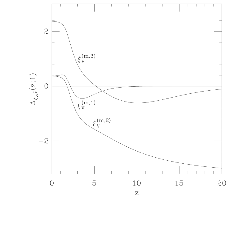
Figure 4: $\Delta_{\xi_{V},2}(z;1)$ for $H^{std}$ for the three different definitions of second-moment correlation length.

Let us now consider the corrections to scaling. The term proportional to $\log L/L^{2}$ is identical in all cases to $\Delta_{m,1}(z;\rho)$, cf. Eq. (3.4). The contribution proportional to $1/L^{2}$ depend instead on the definition of $\xi$. In Figs. 4 and 5 we report the deviations from FSS for the three definitions for the standard and the Symanzik hamiltonians ($\Delta_{\xi,1}$ and $\Delta_{\xi,2}$ are defined in analogy with Eq. (3.2)). Notice that for $\xi^{(m,1)}_{V}$ and $\xi^{(m,3)}_{V}$ the corrections proportional to $1/L^{2}$ do not vanish even when $\alpha_{1}={1\over 12}$, $\alpha_{2}=0$ and Eq. (3.9) are satisfied. This is expected since the second-moment correlation length is an off-shell quantity. Therefore the definition of the correlation length must be improved, as well as the hamiltonian. For instance, if one uses $\xi^{(m,1)}_{V}$ and the Symanzik hamiltonian one does not see any improvement: this definition has large corrections to scaling, and the behaviour is worse for the Symanzik hamiltonian than for the standard one. In this case there is a simple remedy to the problem: modify the definition in such a way that $\xi(L,T)\approx\xi_{\infty}+O(L^{-4},T^{-4},L^{-2}T^{-2})$. Analogously one could proceed for $\xi^{(m,3)}_{V}$. The second definition is automatically improved but this is a peculiarity of the large-$N$ limit.

Let us finally discuss the mass gap $\mu_{V}(L)$ and the exponential correlation length $\xi^{(exp)}_{V}=1/\mu_{V}(L)$. We have computed the FSS functions expressing them in terms of $\mu_{V}(L)$ itself, i.e. using as variable $x\equiv\mu_{V}(L)L$ instead of $z$. We get

$$\left({\mu_{V}(\infty)\over\mu_{V}(L)}\right)^{2}=f_{m}(x;\infty)\left(1+{\Delta_{\mu,1}(x;\infty)\over L^{2}}\log L+{\Delta_{\mu,2}(x;\infty)\over L^{2}}\right)\;,$$ (3.50)

where $\Delta_{\mu,1}(x;\infty)=\Delta_{m,1}(x;\infty)$ and

$$\Delta_{\mu,2}(x;\infty) = \Delta_{m,2}(x;\infty)+{\pi x^{3}\over 6}(12\alpha_{1}+12\alpha_{2}-1){\partial F_{0}\over\partial x}(x;\infty)$$ (3.51)

$$\quad+{8\over 3}(12\alpha_{1}+12\alpha_{2}-1)e^{-4\pi F_{0}(x;\infty)}\;.$$

Thus only the $1/L^{2}$ term differs from the expansion of $m^{2}_{\infty}/m^{2}_{L,T}$. The asymptotic behaviour for large $x$ is analogous to (3.20) while for $x\to 0$ we have

$$\Delta_{\mu,2}(x;\infty)={\pi^{2}\over 18}(12\alpha_{1}-1)-{\pi x\over 3}(12\alpha_{1}+12\alpha_{2}-1)+O(x^{2}).$$ (3.52)

Notice that, since this quantity is defined on-shell, it is improved once the hamiltonian is improved.

3.2.2 Isotensor sector

Let us now consider the isotensor observables. The calculation of the FSS function for the isotensor susceptibility $\chi_{T}$ is straightforward. We obtain

$${\chi_{T}(L,T)\over\chi_{T}(\infty)}\,=\,f_{\chi_{T}}(z;\rho)\left(1+{\Delta_{\chi_{T},1}(z;\rho)\over L^{2}}\log L+{\Delta_{\chi_{T},2}(z;\rho)\over L^{2}}\right),$$ (3.53)

with corrections of order $\log^{2}L/L^{4}$ where

$$\hskip-20.0ptf_{\chi_{T}}(z;\rho) = -{64\pi\over z}{\partial F_{0}\over\partial z}(z;\rho)e^{-4\pi F_{0}(z;\rho)},$$ (3.54)

$$\hskip-20.0pt\Delta_{\chi_{T},1}(z;\rho) = {1\over 4}(12\alpha_{1}+16\alpha_{2}-1)\left[64e^{-4\pi F_{0}(z;\rho)}-z^{2}+{z\over 2\pi}\left({\partial F_{0}\over\partial z}(z;\rho)\right)^{-1}\right]\;,$$ (3.55)

$$\hskip-20.0pt\Delta_{\chi_{T},2}(z;\rho) = 32\pi(12\alpha_{1}+16\alpha_{2}-1)F_{0}(z;\rho)e^{-4\pi F_{0}(z;\rho)}$$ (3.56)

$$-4(28\alpha_{1}+32\alpha_{2}-3)e^{-4\pi F_{0}(z;\rho)}-4\pi{\cal F}_{1}(z;\rho)$$

$$+{\partial{\cal F}_{1}/\partial z(z;\rho)\over\partial F_{0}/\partial z(z;\rho)}-256\pi\Lambda_{1}e^{-4\pi F_{0}(z;\rho)}\;.$$

As before the $\log L/L^{2}$ corrections cancel if $12\alpha_{1}+16\alpha_{2}-1=0$. The function $\Delta_{\chi_{T},2}(z;\rho)$ simplifies considerably if $\alpha_{1}={\textstyle\frac{1}{12}}$ and $\alpha_{2}=0$ . In this case

$$\Delta_{\chi_{T},2}(z;\rho)\,=\,\left({1\over 96\pi}-\Lambda_{1}\right)\left[256\pi e^{-4\pi F_{0}(z;\rho)}-4\pi z^{2}+2z\left({\partial F_{0}\over\partial z}(z;\rho)\right)^{-1}\right]\;.$$ (3.57)

Therefore, if Eq. (3.9) is satisfied, $\chi_{T}$ has only corrections of order $\log L/L^{4}$. It is straightforward to compute the expansions of the various FSS functions in the limit $z\to\infty$. Using the results of Sect. B.2.1 and B.2.2 we obtain

$$f_{\chi_{T}}(z;\rho) = 1+\sqrt{2\pi z}\ e^{-z}+\sqrt{2\pi\rho z}\ e^{-\rho z}+O(z^{-1/2}e^{-z},z^{-1/2}e^{-\rho z}),$$ (3.58)

$$\Delta_{\chi_{T},1}(z;\rho) = {z^{2}\over 4}(12\alpha_{1}+16\alpha_{2}-1)\left(\sqrt{2\pi z}\ e^{-z}+\sqrt{2\pi\rho z}\ e^{-\rho z}\right)$$ (3.59)

$$\qquad\qquad+O(z^{3/2}e^{-z},z^{3/2}e^{-\rho z}),$$

$$\Delta_{\chi_{T},2}(z;\rho) = -{\pi z^{4}\over 12}(12\alpha_{1}+12\alpha_{2}-1)\left({e^{-z}\over\sqrt{2\pi z}}+{\rho^{2}e^{-\rho z}\over\sqrt{2\pi\rho z}}\right)$$ (3.60)

$$-{z^{2}\over 8}(12\alpha_{1}+16\alpha_{2}-1)\,\log{z^{2}\over 32}\,\left(e^{-z}\sqrt{2\pi z}+e^{-\rho z}\sqrt{2\pi\rho z}\right)$$

$$\qquad\qquad+O(z^{5/2}e^{-z},z^{5/2}e^{-\rho z}).$$

As expected, $f_{\chi_{T}}(z;\rho)$ behaves as $z^{p}e^{-z}$, but $p$ differs from the value it assumes for other observables (see e.g. the large-$z$ behaviour of $\chi_{V}$). Indeed, while the exponential behaviour is completely general, the power $p$ depends on the observable.

In Figs. 6 and 7 we report the graphs of $\Delta_{\chi_{T},1}(z;\rho)$ and $\Delta_{\chi_{T},2}(z;\rho)$ for $\rho=1$ and different hamiltonians. The behaviour is very similar to the behaviour of $m^{2}_{L,T}/m^{2}_{\infty}$. The FSS corrections are quite small. The Symanzik hamiltonian shows the best behaviour, while the diagonal hamiltonian is the one with the largest deviations from FSS.

Finally let us compute the FSS curve for the tensor correlation length. We will restrict the discussion to the standard action; the generalization to generic hamiltonians is straightforward but the final expressions are cumbersome. Moreover we will restrict our discussion to $\xi^{(m,1)}_{T}$, that is to the definition used in numerical simulations. We obtain

$$\left({\xi_{T}^{(m,1)}(L,T)\over\xi_{T}^{(m)}(\infty)}\right)^{2}\,=\,f_{\xi_{T}}(z;\rho)\left(1+{\Delta_{\xi_{T},1}(z;\rho)\over L^{2}}\log L+{\Delta_{\xi_{T},2}(z;\rho)\over L^{2}}\right),$$ (3.61)

where

$$\hskip-20.0ptf_{\xi_{T}}(z;\rho) = 192\ \Xi_{1}(z;\rho)e^{-4\pi F_{0}(z;\rho)},$$ (3.62)

$$\hskip-20.0pt\Delta_{\xi_{T},1}(z;\rho) = \Delta_{m,1}(z;\rho)+{\Xi_{2}(z;\rho)\over\Xi_{1}(z;\rho)}+8e^{-4\pi F_{0}(z;\rho)},$$ (3.63)

$$\hskip-20.0pt\Delta_{\xi_{T},2}(z;\rho) = \Delta_{m,2}(z;\rho)+{\Xi_{3}(z;\rho)\over\Xi_{1}(z;\rho)}-4e^{-4\pi F_{0}(z;\rho)}+16\pi F_{0}(z;\rho)e^{-4\pi F_{0}(z;\rho)},$$ (3.64)

and

$$\hskip-20.0pt\Xi_{1}(z;\rho) = {1\over 8\pi^{2}}\left[-1-\rho^{2}-{1\over 2z}{\partial F_{0}\over\partial z}(z;\rho)\left({1\over F_{3}(z;\rho)}+{1\over F_{3}(\rho z;1/\rho)}\right)\right]\;,$$ (3.65)

$$\hskip-20.0pt\Xi_{2}(z;\rho) = {1\over 128\pi^{3}}\left[{1\over F_{3}(z;\rho)}+{1\over F_{3}(\rho z;1/\rho)}\right.$$ (3.66)

$$\quad\left.+{1\over 2z}{\partial F_{0}\over\partial z}(z;\rho)\left({1\over F_{3}^{2}(z;\rho)}+{1\over\rho^{2}F_{3}^{2}(\rho z;1/\rho)}\right)\right]\;,$$

$$\hskip-20.0pt\Xi_{3}(z;\rho) = {1\over 8\pi^{2}}\left[-{1\over 2z}{\partial F_{1}\over\partial z}(z;\rho)\left({1\over F_{3}(z;\rho)}+{1\over F_{3}(\rho z;1/\rho)}\right)\right.$$ (3.67)

$$-{2\pi^{2}\over 3}-{\pi^{2}\over 6z}{\partial F_{0}\over\partial z}(z;\rho)\left({1\over F_{3}(z;\rho)}+{1\over\rho^{2}F_{3}(\rho z;1/\rho)}\right)$$

$$\left.+{1\over 2z}{\partial F_{0}\over\partial z}(z;\rho)\left({F_{4}(z;\rho)\over F_{3}^{2}(z;\rho)}+{F_{4}(\rho z;1/\rho)\over\rho^{2}F_{3}^{2}(\rho z;1/\rho)}+{1\over 16\pi}{\log\rho\over\rho^{2}F_{3}^{2}(\rho z;1/\rho)}\right)\right].$$

Using Eqs. (B.57), (LABEL:F1largez), (B.106), and (B.107) it is straightforward to compute the large-$z$ behaviour of the various FSS functions. We obtain

$$\hskip-10.0ptf_{\xi_{T}}(z;\rho) = 1-{\pi^{2}\over 15z^{2}}{1+\rho^{2}\over\rho^{2}}+{2\pi^{4}\over 63z^{4}}{1+\rho^{4}\over\rho^{4}}+O(z^{-6}),$$ (3.68)

$$\hskip-10.0pt\Delta_{\xi_{T},1}(z;\rho) = -{\pi^{2}\over 12}{1+\rho^{2}\over\rho^{2}}+{\pi^{4}\over 180\rho^{4}z^{2}}(3-2\rho^{2}+3\rho^{4})+O(z^{-4}),$$ (3.69)

$$\hskip-10.0pt\Delta_{\xi_{T},2}(z;\rho) = {\pi^{2}\over 24\rho^{2}}(1+\rho^{2})\left(\log{z^{2}\over 32}+4\right)$$ (3.70)

$$\hskip-30.0pt-{\pi^{4}\over 360\rho^{4}z^{2}}(3-2\rho^{2}+3\rho^{4})\log{z^{2}\over 32}-{\pi^{4}\over 90\rho^{4}z^{2}}(1-\rho^{2})^{2}+O(\log z/z^{4}).$$

As expected $f_{\xi_{T}}(z;\rho)$ approaches one as $1/z^{2}$ and thus it reaches the asymptotic value for $z\to\infty$ within 1% only for $z\approx 9$. Notice moreover that $\Delta_{\xi_{T},2}(z;\rho)$ diverges logarithmically as $z\to\infty$. This fact signals the non-uniformity of the expansion in $z$. This is not unexpected. Indeed, for each fixed $z$, we expect the expansion to be reliable only if $m_{L,T}\ll 1$, i.e. if the correlation length is much larger than a lattice spacing. Therefore we expect the expansion to be valid only if $z\ll L$. If $1\ll z\ll L$, $\log z/L^{2}$ is a small number and thus the expansion is completely under control.

The functions $\Delta_{\xi_{T},1}(z;\rho)$ and $\Delta_{\xi_{T},2}(z;\rho)$ are reported for $\rho=1$ in Figs. 6 and 8. From these plots, comparing with the analogous graphs for other observables, one can immediately see that the corrections to FSS for $\xi^{(m,1)}_{T}$ are quite large. This is particularly evident in the large-$z$ region, where the $\log L/L^{2}$ term goes to a constant (for the isovector correlation length this term vanishes exponentially), while the $1/L^{2}$ term diverges as $\log z$.

4 Mixed $O(N)$-$RP^{N-1}$ model

In this section we compute the FSS corrections for the hamiltonian (2.18). As before we want to obtain a relation between $m_{\infty}^{2}$ and $m^{2}_{L,T}$ at fixed $\beta$. Using now the gap equation (2.19) we have

$${4I_{L,T}(m_{L,T}^{2})^{2}\over 4I_{L,T}(m_{L,T}^{2})+r(m^{2}_{L,T}I_{L,T}(m^{2}_{L,T})-1)}={4I_{\infty}(m_{\infty}^{2})^{2}\over 4I_{\infty}(m_{\infty}^{2})+r(m^{2}_{\infty}I_{\infty}(m^{2}_{\infty})-1)}\;.$$ (4.1)

We will now discuss the FSS limit in which $L,T\to\infty$, $\beta\to\infty$, $m_{L,T},m_{\infty}\to 0$ with $m_{L,T}L\equiv z$ and $T/L\equiv\rho$ fixed. At leading order we can disregard the terms $m^{2}_{\infty}I_{\infty}(m^{2}_{\infty})$ and $m^{2}_{L,T}I_{L,T}(m^{2}_{L,T})$ in the denominators obtaining

$${I_{L,T}(m_{L,T}^{2})^{2}\over 4I_{L,T}(m_{L,T}^{2})-r}={I_{\infty}(m_{\infty}^{2})^{2}\over 4I_{\infty}(m_{\infty}^{2})-r}\;,$$ (4.2)

that implies $I_{L,T}(m_{L,T}^{2})=I_{\infty}(m_{\infty}^{2})$. Thus, at leading order, the relation between $m_{L,T}$ and $m_{\infty}$ is identical to the one we have discussed in the previous section. Consequently the FSS functions for the hamiltonian (2.18) are identical to the FSS functions of models with hamiltonian (2.1), as expected on the basis of universality. The corrections will however be different. Writing

$$I_{\infty}(m_{\infty}^{2})=I_{L,T}(m_{L,T}^{2})+\delta\ m_{L,T}^{2}\;,$$ (4.3)

a simple computation gives

$$\delta={r\over 2}\left({m_{\infty}^{2}\over m_{L,T}^{2}}-1\right)\ {I_{L,T}(m_{L,T}^{2})^{2}\over 2I_{L,T}(m_{L,T}^{2})-r}\;.$$ (4.4)

Solving for $m_{\infty}^{2}/m_{L,T}^{2}$ we get finally

$${m_{\infty}^{2}\over m_{L,T}^{2}} = f_{m}(z;\rho)\left(1+{(\Delta_{m,1}(z;\rho)+\Delta_{m,1}^{r}(z;\rho))\over L^{2}}\log L+{(\Delta_{m,2}(z;\rho)+\Delta_{m,2}^{r}(z;\rho))\over L^{2}}+\right.$$ (4.5)

$$+\left.{\widehat{\Delta_{m}^{r}}(L;z;\rho)\over L^{2}}\right)\;,$$

where $f_{m}(z;\rho)$, $\Delta_{m,1}(z;\rho)$ and $\Delta_{m,2}(z;\rho)$ are defined in Eqs. (3.3), (3.4) and (3.5), with $\alpha_{1}=\alpha_{2}=0$ and

$$\Delta_{m,1}^{r}(z;\rho) = {r\over 2}\left(z^{2}-32e^{-4\pi F_{0}(z;\rho)}\right),$$ (4.6)

$$\Delta_{m,2}^{r}(z;\rho) = {\pi r\over 2}\left(2F_{0}(z;\rho)+r\right)\left(z^{2}-32e^{-4\pi F_{0}(z;\rho)}\right),$$ (4.7)

$$\widehat{\Delta_{m}^{r}}(L;z;\rho) = {\pi^{2}r^{3}\over 2}\left(z^{2}-32e^{-4\pi F_{0}(z;\rho)}\right)\,{1\over\log L+2\pi F_{0}(z;\rho)-\pi r}\;.$$ (4.8)

The result (4.5) is quite different from Eq. (3.2). Indeed, while before the corrections had a very simple dependence on $\log L$, now the corrections involve $\widehat{\Delta_{m}^{r}}(L;z;\rho)$ that is not a simple polynomial in $\log L$. Notice that, for large $L$ at fixed $z$, $\widehat{\Delta_{m}^{r}}(L;z;\rho)$ behaves as $1/\log L$. Therefore, in the FSS limit, the corrections still behave as $\log L/L^{2}$.

We should make a second remark about $\widehat{\Delta_{m}^{r}}(L;z;\rho)$. It is easy to convince oneself from the asymptotic expansions, Eqs. (B.57), (B.59), and (B.69), that $F_{0}(z;\rho)$ assumes any real value. Therefore, for each value of $L$, there is a value $z_{c}$ such that the denominator in Eq. (4.8) vanishes, and therefore $\widehat{\Delta_{m}^{r}}(L;z;\rho)$ diverges. When $L\to\infty$, $z_{c}\to\infty$; more precisely, using Eq. (B.57), we have $z_{c}\approx e^{-\pi r}\sqrt{32}L$. This singularity is a signal of the fact that the expansion is not uniform in $z$. For each $z$ the expansion is valid only when $L\gg z$, i.e. for $m_{L,T}\ll 1$. In other words the expansion makes sense only when the correlation length is much larger than a lattice spacing.

$L$	$R_{exact}(L;2,1)$	$R_{expan}(L;2,1)$	$D_{exact}(L;2,1)$	$D_{expan}(L;2,1)$
8	0.35709886	0.34256990	0.5916549	0.5268967
10	0.29398737	0.29002279	0.3103555	0.2926846
12	0.26809044	0.26656021	0.1949281	0.1881076
14	0.25463070	0.25391316	0.1349356	0.1317374
16	0.24665643	0.24627448	0.0993928	0.0976904
32	0.22943124	0.22941299	0.0226170	0.0225356
64	0.22561220	0.22561112	0.0055948	0.0055900
128	0.22467784	0.22467777	0.0014302	0.0014300
$\infty$		0.22435696

Table 3: Values of $R_{exact}(L;z,\rho)$, $R_{expan}(L;z,\rho)$, $D_{exact}(L;z,\rho)$, and $D_{expan}(L;z,\rho)$ for the $RP^{\infty}$ model ($r=1$), $\rho=1$ and $z=2$.

The corrections are larger for the mixed model than for the vector model. For instance $\Delta^{r}_{m,1}(z;\rho)/\Delta_{m,1}(z;\rho)=2r$ so that the logarithmic correction in the $RP^{\infty}$ model ($r=1$) is three times larger than the corresponding one in the $N$-vector model ($r=0$). For the values of $L$ that are used in Monte Carlo simulations, say $8\leq L\leq 128$, however all terms in Eq. (4.5) contribute to the FSS corrections. In table 3 we report for $r=1$, $\rho=1$ and $z=2$, the same quantities reported in table 1. Comparing the two tables we see that the corrections to FSS for $RP^{\infty}$ are seven times larger than those for the $N$-vector model in the same range of values of $L$. Only for $L\approx 50$ (resp. $L\approx 150$) the corrections are smaller than 1% (resp. 0.1%). To compare the corrections for the $RP^{\infty}$ and the $N$-vector model with the standard hamiltonian for all values of $z$, in Fig. 9 we report

$$S(L;z;\rho)={D_{expan}(L;z,\rho)_{r=1}\over D_{expan}(L;z,\rho)_{r=0}}$$ (4.9)

for $L=128,512$ and $\rho=1$ ($D(L;z,\rho)$ is defined in Eq. (3.17)). For these values of $L$, corrections are 5-10 times larger in the $RP^{\infty}$ model.

It is interesting to understand the origin of $\widehat{\Delta_{m}^{r}}(L;z;\rho)$ in terms of perturbation theory. First of all, for $z$ small, (for simplicity we consider the strip case, analogous results are valid for generic $\rho$) we can expand, cf. Eq. (B.69),

$$\widehat{\Delta_{m}^{r}}(L;z;\rho)={\pi^{2}r^{3}\over 2}{z^{3}\over\pi+z\log L}\left[1-{\pi z(2\overline{F}_{00}-r)\over\pi+z\log L}+O(z^{2})\right].$$ (4.10)

This is not yet a perturbative expansion in $z$ due to the presence of the term $z\log L$ in the denominators. This term cannot be expanded in $z$ since we are considering an asymptotic expansion at fixed $z$ with $L\to\infty$. However, if we ignore this problem and expand the denominators in powers of $z$, we obtain

$$\widehat{\Delta_{m}^{r}}(L;z;\rho)_{pert}={\pi r^{3}\over 2}z^{3}\left(1-{z\over\pi}\log L-z(2\overline{F}_{00}-r)+O(z^{2}\log^{2}L)\right).$$ (4.11)

In general $\widehat{\Delta_{m}^{r}}(L;z;\rho)$ has a polynomial expansion in $z$ with coefficients that are polynomials in $\log L$:

$$\widehat{\Delta_{m}^{r}}(L;z;\rho)_{pert}=z^{3}\sum_{n=0}^{\infty}P_{n}(\log L)z^{n},$$ (4.12)

where $P_{n}(x)$ is a polynomial of degree $n$. This expansion is clearly incorrect in the FSS limit $L\to\infty$ at fixed $z$. However Eq. (4.12) correctly describes the theory in the limit $z\to 0$ at fixed $L$. This is the limit in which PT works correctly [44, 45], and indeed the expansion (4.12) can be directly obtained with a perturbative calculation. Therefore our results show that in order to correctly compute the corrections to FSS one needs to resum the perturbative expansion. This reflects the fact that the perturbative limit $z\to 0$ with $L$ large and fixed does not commute with the FSS limit $L\to\infty$ with $z$ fixed and small. It should also be noticed that the infinite series of logarithms appearing in Eq. (4.12) resums to give corrections of order $1/(L^{2}\log L)$. This is a result far from obvious: in general one expects series of the form (4.12) to give powers of $L$, i.e. to resum to $L^{p(z)}$, where $p(z)$ is some function of $z$. For $N=\infty$ no power is generated, but we have no proof that this will be true for generic values of $N$. The only argument we have against the appearance of power corrections is based on a naive application of renormalization-group ideas. The corrections to FSS are due to the irrelevant operators of the theory. Since the $N$-vector model is asymptotically free, operators have canonical scaling dimensions with logarithmic corrections. Therefore we always expect a behaviour of the form $(\log L)^{p}/L^{2}$.

Using the results of the previous section it is easy to obtain the FSS functions and their leading corrections for the various observables. For the isovector second-moment correlation lengths the expressions (3.31), (LABEL:xim2FSS) and (3.33) still hold with $m_{\infty}^{2}/m_{L,T}^{2}$ given by Eq. (4.5). For the susceptibility $\chi_{V}$ we have

$${\chi_{V}(L,T)\over\chi_{V}(\infty)}\,=\,{m_{\infty}^{2}\over m_{L,T}^{2}}\left[1+{r\over 4z^{2}L^{2}}\left(32e^{-4\pi F_{0}(z;\rho)}-z^{2}\right){\log L+2\pi F_{0}(z;\rho)\over\log L+2\pi F_{0}(z;\rho)-\pi r}\right]\;,$$ (4.13)

while for $\chi_{T}$ we have

$${\chi_{T}(L,T)\over\chi_{T}(\infty)} = \left({\chi_{T}(L,T)\over\chi_{T}(\infty)}\right)_{r=0}\left[1+{\Delta_{m,1}^{r}(z;\rho)\over L^{2}}\log L+{\Delta_{m,2}^{r}(z;\rho)\over L^{2}}+{\widehat{\Delta_{m}^{r}}(L;z;\rho)\over L^{2}}\right.$$ (4.14)

$$\left.+{r\over 2z^{2}L^{2}}\left(32e^{-4\pi F_{0}(z;\rho)}-z^{2}\right){\log L+2\pi F_{0}(z;\rho)\over\log L+2\pi F_{0}(z;\rho)-\pi r}\right]\;.$$

Finally for $\xi_{T}^{(m,1)}$ we have

$$\left({\xi^{(m,1)}_{T}(L,T)\over\xi^{(m,1)}_{T}(\infty)}\right)^{2}=\ \left({\xi^{(m,1)}_{T}(L,T)\over\xi^{(m,1)}_{T}(\infty)}\right)_{r=0}^{2}\left[1+{\Delta_{m,1}^{r}(z;\rho)\over L^{2}}\log L+{\Delta_{m,2}^{r}(z;\rho)\over L^{2}}+{\widehat{\Delta_{m}^{r}}(L;z;\rho)\over L^{2}}\right].$$ (4.15)

To conclude our discussion we come back again to the $RP^{\infty}$ model. In this case the FSS functions are usually reported in terms of $s=L/\xi_{T}^{(m,1)}(L,T)$. Indeed, because of the gauge symmetry, one cannot define observables in the isovector sector. For any observable $\cal O$, we define the FSS deviations

$$\overline{D}_{\cal O}(L;s;\rho)=L^{2}\left[{{\cal O}(L,T)\over{\cal O}(\infty)}{1\over\overline{f}_{\cal O}(s;\rho)}-1\right].$$ (4.16)

where $\overline{f}_{\cal O}(s;\rho)$ is the FSS function of ${\cal O}$ expressed in terms of $s$. In Figs. 10 and 11 we report $\overline{D}_{\xi_{T}}(L;z;1)$ and $\overline{D}_{\chi_{T}}(L;z;1)$ for $L=16$ and $L=128$. The corrections are extremely large if one compares them with the analogous results for the $N$-vector model. This is especially true in the large-$s$ region. Moreover the corrections are positive. These results are in qualitative agreement with the results of Ref. [47].

5 Conclusions

In this paper we have investigated the corrections to FSS in the large-$N$ limit for a vast class of models and we have studied their relation with the improvement program of Symanzik.

In the large-$N$ limit we find that the corrections behave as $f(z,L)\log L/L^{2}$ where $f(z,L)$ can be expanded in powers of $1/\log L$ and is such that $f(z,\infty)$ is finite for all values of $z$. Thus, for large values of $L$, corrections behave as $\log L/L^{2}$. Tree-level improved hamiltonians have corrections to FSS behaving as $1/L^{2}$: the effect of the improvement is the cancellation of a logarithm. Subsequent perturbative improvement should give hamiltonians with corrections of order $1/(L^{2}\log^{l}L)$ ($l=1$ for one-loop improvement and so on).

We have shown explicitly that the FSS limit and the perturbative limit commute in the calculations of the FSS functions but not for the calculation of the next-to-leading term. Corrections to FSS cannot be computed in perturbation theory unless an infinite series of logarithms is resummed.

Finally we have investigated if there is any sign of large correction in the $RP^{\infty}$ model. We find that this model shows deviations from FSS that are much larger than those of the $N$-vector model. We find qualitative agreement with the results of Ref. [47].

Appendix A Definitions

A.1 Functions $G_{k}(\alpha)$, $H_{k}(\alpha)$ and ${\cal H}_{k}(\alpha)$

Let us define the following functions:

$$G_{k}(\alpha) = \sum_{n=1}^{\infty}\left[(n^{2}+\alpha^{2})^{k-1/2}-\sum_{m=0}^{k}{k-1/2\choose m}\alpha^{2m}n^{2k-2m-1}\right]\;,$$ (A.1)

$$H_{k}(\alpha) = \sum_{n=1}^{\infty}{1\over(n^{2}+\alpha^{2})^{k+1/2}}\;,$$ (A.2)

$${\cal H}_{k}(\alpha) = \sum_{n=1}^{\infty}{1\over(1-4n^{2})(n^{2}+\alpha^{2})^{k+1/2}}\;.$$ (A.3)

The first and the third ones are defined for integers $k\geq 0$ while the second one is defined for $k\geq 1$: for these values of $k$ the sums converge for all values of $\alpha$. The functions $G_{k}(\alpha)$ and $H_{k}(\alpha)$ are known in statistical mechanics under the name of remnant functions (see App. D of Ref. [39] and Ref. [51]).

We want now to discuss their behaviour for $\alpha\to 0$ and $\alpha\to\infty$. We will focus on those values of $k$ that appear in our final results, i.e. to $k=0,1$.

The expansion for $\alpha\to 0$ is trivial. We obtain

$$G_{0}(\alpha) = \sum_{k=1}^{\infty}(-1)^{k}{2k\choose k}\zeta(2k+1)\left({\alpha\over 2}\right)^{2k},$$ (A.4)

$$G_{1}(\alpha) = 2\sum_{k=1}^{\infty}{(-1)^{k}\over k}{2k\choose k}\zeta(2k+1)\left({\alpha\over 2}\right)^{2k+2},$$ (A.5)

$$H_{1}(\alpha) = \sum_{k=0}^{\infty}(-1)^{k}(2k+1){2k\choose k}\zeta(2k+3)\left({\alpha\over 2}\right)^{2k},$$ (A.6)

$${\cal H}_{0}(\alpha) = \sum_{k=0}^{\infty}(-1)^{k}{2k\choose k}\alpha^{2k}\left[1-2\log 2+\sum_{n=1}^{k}{\zeta(2n+1)\over 4^{n}}\right]\;,$$ (A.7)

$${\cal H}_{1}(\alpha) = 4\sum_{k=0}^{\infty}(-1)^{k}(2k+1){2k\choose k}\alpha^{2k}\left[1-2\log 2+\sum_{n=1}^{k+1}{\zeta(2n+1)\over 4^{n}}\right]\;,$$ (A.8)

where we have used

$$\sum_{n=1}^{\infty}{1\over(1-4n^{2})n^{2q+1}}\,=\,4^{q}(1-2\log 2)+\,4^{q}\sum_{s=1}^{q}{\zeta(2s+1)\over 4^{s}}\;.$$ (A.9)

All series converge for $|\alpha|<1$.

We want now to derive the asymptotic expansions for $\alpha\to\infty$. In order to obtain them let us derive a different representation for the functions $G_{k}(\alpha)$ and $H_{k}(\alpha)$.

Let us first consider $G_{0}(\alpha)$. We rewrite it as

$$G_{0}(\alpha)=\lim_{\epsilon\to 0+}\left[-\zeta(1+\epsilon)+{1\over\Gamma(1/2+\epsilon/2)}\int^{\infty}_{0}{dx\over x^{(1-\epsilon)/2}}e^{-x\alpha^{2}}\sum_{n=1}^{\infty}e^{-xn^{2}}\right]\;.$$ (A.10)

Using the Poisson resummation formula [66] we obtain

$$G_{0}(\alpha) = \lim_{\epsilon\to 0+}\left\{-\zeta(1+\epsilon)+{\alpha^{-\epsilon}\over\Gamma(1/2+\epsilon/2)}\left({\sqrt{\pi}\over 2}\Gamma\left({\epsilon\over 2}\right)-{1\over 2\alpha}\Gamma\left({1+\epsilon\over 2}\right)\right)\right.$$ (A.11)

$$\qquad\left.+{\sqrt{\pi}\over\Gamma(1/2+\epsilon/2)}\int_{0}^{\infty}{dx\over x^{1-\epsilon/2}}e^{-x\alpha^{2}}\sum_{n=1}^{\infty}\exp\left(-{\pi^{2}n^{2}\over x}\right)\right\}\;.$$

Taking the limit we get the representation [51]

$$G_{0}(\alpha)=-\log{\alpha\over 2}-\gamma_{E}-{1\over 2\alpha}+2\sum_{n=1}^{\infty}K_{0}(2\pi n\alpha),$$ (A.12)

where $K_{0}$ is a modified Bessel function [67]. The corresponding representations for $G_{k}(\alpha)$ and $H_{k}(\alpha)$, $k\geq 1$ can be obtained by integration and derivation of the previous relation. We obtain [51]

$$G_{1}(\alpha) = {1\over 12}+{\alpha^{2}\over 2}\left(-\log{\alpha\over 2}+{1\over 2}-\gamma_{E}-{1\over\alpha}\right)-{\alpha\over\pi}\sum_{n=1}^{\infty}{1\over n}K_{1}(2\pi n\alpha),$$ (A.13)

$$H_{1}(\alpha) = {1\over\alpha^{2}}-{1\over 2\alpha^{3}}+{4\pi\over\alpha}\sum_{n=1}^{\infty}nK_{1}(2\pi n\alpha).$$ (A.14)

This representation of the functions $G_{k}(\alpha)$ and $H_{k}(\alpha)$ allows an immediate derivation of the asymptotic expansion for large values of $\alpha$ since [67]

$$K_{n}(x)=\sqrt{{\pi\over 2x}}e^{-x}\left[1+{1\over 2x}\left(n^{2}-{1\over 4}\right)+O(x^{-2})\right]\;\;.$$ (A.15)

Let us now consider the functions ${\cal H}_{k}(\alpha)$. We rewrite ${\cal H}_{k}(\alpha)$ as

$${\cal H}_{k}(\alpha)\,=\,-{1\over 2}{1\over\alpha^{2k+1}}+{1\over 2}{1\over\Gamma(k+1/2)}\int^{\infty}_{0}dx\,x^{k-1/2}e^{-x\alpha^{2}}g(x),$$ (A.16)

where

$$g(x)=\,\sum_{n=-\infty}^{+\infty}{e^{-xn^{2}}\over{1-4n^{2}}}\;.$$ (A.17)

Now in the integral appearing in Eq. (A.16) the relevant region for large $\alpha^{2}$ corresponds to small values of $x$. Therefore we need the small-$x$ expansion of $g(x)$. First of all notice that

$$g(0)=1+2\sum_{n=1}^{+\infty}{1\over 1-4n^{2}}=0.$$ (A.18)

Then one immediately verifies that $g(x)$ satisfies an equation of the form

$$g^{\prime}(x)+{1\over 4}g(x)-{1\over 4}\sum_{n=-\infty}^{+\infty}e^{-xn^{2}}=0,$$ (A.19)

so that, using Eq. (A.18), we get

$$g(x)={1\over 4}e^{-x/4}\int_{0}^{x}dy\ e^{y/4}\sum_{n=-\infty}^{+\infty}e^{-yn^{2}}.$$ (A.20)

Using the Poisson resummation formula [66] we can rewrite it as

$$g(x)={\sqrt{\pi}\over 4}e^{-x/4}\int_{0}^{x}{dy\over\sqrt{y}}\ e^{y/4}\sum_{n=-\infty}^{+\infty}e^{-\pi^{2}n^{2}/y}.$$ (A.21)

In the small-$x$ region only the term with $n=0$ is relevant so that

$$g(x) \approx {\sqrt{\pi}\over 4}e^{-x/4}\int_{0}^{x}{dy\over\sqrt{y}}\ e^{y/4}$$ (A.22)

$$\approx {\sqrt{\pi x}\over 2}\left(1-{x\over 6}+{x^{2}\over 60}-{x^{3}\over 840}+{x^{4}\over 15120}+O(x^{5})\right)\;.$$

We obtain eventually for large values of $\alpha$

$${\cal H}_{k}(\alpha) = -{1\over 2}{1\over\alpha^{2k+1}}+\,{\sqrt{\pi}\over 4\ \Gamma(k+1/2)}{1\over\alpha^{2k+2}}\times$$

$$\left[k!-{(k+1)!\over 6\alpha^{2}}+{(k+2)!\over 60\alpha^{4}}-{(k+3)!\over 840\alpha^{6}}+{(k+4)!\over 15120\alpha^{8}}\right]+O(\alpha^{-2k-12}).$$

A.2 The functions $M_{pq}(z;\rho)$, $N_{pq}(\rho)$, ${\cal M}_{pq}(z;\rho)$ and ${\cal N}_{pq}(\rho)$

A second set of functions appear in our calculations. We define

$$\hskip-60.0ptM_{pq}(z;\rho) = (2\pi)^{p}\sum_{n=-\infty}^{\infty}{1\over(4\pi^{2}n^{2}+z^{2})^{p/2}}{1\over[\exp(\rho\sqrt{4\pi^{2}n^{2}+z^{2}})-1]^{q}},$$ (A.24)

$$\hskip-60.0pt{\cal M}_{pq}(z;\rho) = (2\pi)^{p}\sum_{n=-\infty}^{\infty}{1\over(1-4n^{2})(4\pi^{2}n^{2}+z^{2})^{p/2}}{1\over[\exp(\rho\sqrt{4\pi^{2}n^{2}+z^{2}})-1]^{q}},$$ (A.25)

$$\hskip-60.0ptN_{pq}(\rho) = \sum_{n=1}^{\infty}{1\over n^{p}}{1\over[\exp(2\pi\rho n)-1]^{q}},$$ (A.26)

$$\hskip-60.0pt{\cal N}_{pq}(\rho) = \sum_{n=1}^{\infty}{1\over(1-4n^{2})n^{p}}{1\over[\exp(2\pi\rho n)-1]^{q}},$$ (A.27)

where $q$ is a positive integer. We want to compute here the asymptotic expansion of $M_{pq}(z;\rho)$ and ${\cal M}_{pq}(z;\rho)$ for $z\to 0$ and $z\to\infty$ at fixed $\rho$. The first expansion is straightforward and we get for $M_{pq}(z;\rho)$

$$M_{pq}(z;\rho) = \left({2\pi\over z}\right)^{p}{1\over(\rho z)^{q}}\sum_{n_{1},\ldots,n_{q}=0}^{\infty}{B_{n_{1}}\ldots B_{n_{q}}\over n_{1}!\ldots n_{q}!}(\rho z)^{n_{1}+\ldots+n_{q}}+2N_{pq}(\rho)$$

$$+2z^{2}\left[-{p\over 8\pi^{2}}N_{p+2,q}(\rho)-{q\rho\over 4\pi}\left(N_{p+1,q}(\rho)+N_{p+1,q+1}(\rho)\right)\right]+O(z^{4}).$$

For ${\cal M}_{pq}(z;\rho)$ the expansion is analogous with the substitution of $N_{pq}$ with ${\cal N}_{pq}$.

For large $z$ let us consider first $M_{pq}(z;\rho)$. We obtain

$$M_{pq}(z;\rho)=\,\sum_{n=-\infty}^{\infty}{(2\pi)^{p}\over(4\pi^{2}n^{2}+z^{2})^{p/2}}\exp\left[-q\rho\sqrt{4\pi^{2}n^{2}+z^{2}}\right]+O(e^{-2\rho qz}z^{1/2-p}).$$ (A.29)

This last sum can be evaluated using the Poisson resummation formula [66]. Define

$$\hat{f}(\omega)=\int^{\infty}_{-\infty}dt\,e^{i\omega t}{(2\pi)^{p}\over(4\pi^{2}t^{2}+z^{2})^{p/2}}\exp\left[-q\rho\sqrt{4\pi^{2}t^{2}+z^{2}}\right]\;.$$ (A.30)

Then

$$M_{pq}(z;\rho)\approx\sum_{n=-\infty}^{\infty}\hat{f}(2\pi n).$$ (A.31)

For $z\to\infty$ we have

$$\hat{f}(\omega)={2\pi\over\sqrt{z}}(q\rho z)^{1-p}(\omega^{2}+4\pi^{2}q^{2}\rho^{2})^{(2p-3)/4}\exp\left[-{z\over 2\pi}\sqrt{\omega^{2}+4\pi^{2}q^{2}\rho^{2}}\right]\left(1+O(z^{-1})\right).$$ (A.32)

Therefore

$$M_{pq}(z;\rho)={1\over\sqrt{q\rho}}\left({z\over 2\pi}\right)^{1/2-p}e^{-q\rho z}\left(1+O(z^{-1})\right).$$ (A.33)

For ${\cal M}_{pq}(z;\rho)$ we will not need the explicit asymptotic behaviour. It is however easy to convince oneself that, for large $z$, ${\cal M}_{pq}(z;\rho)$ goes to zero faster than $z^{-p}e^{-q\rho z}$.

To conclude this subsection let us derive a set of relations for the functions $N_{pq}(\rho)$. First of all let us notice that $N_{1,1}(\rho)$ can be related to Dedekind’s $\eta$-function [62]

$$\eta(\tau)=\,e^{\pi i\tau/12}\prod_{n=1}^{\infty}\left(1-e^{2\pi in\tau}\right).$$ (A.34)

Indeed

$$N_{1,1}(\rho) = \sum_{n=1}^{\infty}\sum_{k=1}^{\infty}{1\over n}e^{-2\pi nk\rho}=\,-\log\left[\prod_{k=1}^{\infty}\left(1-e^{-2\pi k\rho}\right)\right]$$ (A.35)

$$= -{\pi\rho\over 12}-\log\eta(i\rho).$$

Following the same steps it is possible to prove that, for $p>0$,

$$N_{-p,1}(\rho)\,=\,{(-1)^{p}\over(2\pi)^{p}}{d^{p}\over d\rho^{p}}N_{p,1}(\rho).$$ (A.36)

This relation, together with

$${d\over d\rho}N_{pq}(\rho)\,=\,-2\pi q\left[N_{p-1,q}(\rho)+N_{p-1,q+1}(\rho)\right]\;,$$ (A.37)

allows to prove that all $N_{pq}(\rho)$ with $p\leq-1$ can be expressed in terms of $N_{0,q^{\prime}}(\rho)$. From Eqs. (A.36) and (A.37) we obtain the following relations we will use in the following:

$$N_{-1,1}(\rho)\,=\,N_{0,1}(\rho)+N_{0,2}(\rho)=\,{1\over 24}+{1\over 2\pi}{d\over d\rho}\log\eta(i\rho),$$ (A.38)

$$N_{-2,1}(\rho)+N_{-2,2}(\rho)\,=\,N_{-1,1}(\rho)+3N_{-1,2}(\rho)+2N_{-1,3}(\rho)\,=\,-{1\over 4\pi^{2}}{d^{2}\over d\rho^{2}}\log\eta(i\rho).$$

Finally, for $p\geq 0$, let us derive a relation between $N_{4p+3,1}(\rho)$ and $N_{4p+3,1}(1/\rho)$ that will allow us to compute explicitly $N_{4p+3,1}(1)$. Let us start from

$$\sum_{n=-\infty}^{\infty}{1\over n^{2}+\alpha^{2}}=\,{\pi\over\alpha}+{2\pi\over\alpha}{1\over e^{2\pi\alpha}-1}.$$ (A.40)

It follows

$$\sum_{m,n=1}^{\infty}\left({1\over n^{4p+2}}+{1\over(\rho m)^{4p+2}}\right)\,{1\over n^{2}+\rho^{2}m^{2}}=$$

$$\qquad-{1\over 2}\zeta(4p+4)+{\pi\over 2\rho}\zeta(4p+3)+\,{\pi\over\rho}N_{4p+3,1}(1/\rho)$$

$$\qquad+{1\over\rho^{4p+2}}\left[-{1\over 2\rho^{2}}\zeta(4p+4)+{\pi\over 2\rho}\zeta(4p+3)+{\pi\over\rho}N_{4p+3,1}(\rho)\right]\;.$$ (A.41)

However, for integer $p\geq 0$, we can also compute the first sum as

$$\sum_{m,n=1}^{\infty}{1\over(nm\rho)^{4p+2}}{n^{4p+2}+(\rho m)^{4p+2}\over n^{2}+(\rho m)^{2}}$$

$$\qquad=\,\sum_{k=0}^{2p}(-1)^{k}\sum_{m,n=1}^{\infty}{1\over(mn\rho)^{4p+2}}(\rho m)^{2k}n^{4p-2k}$$

$$\qquad=\,\sum_{k=0}^{2p}(-1)^{k}{1\over\rho^{4p-2k+2}}\zeta(4p-2k+2)\zeta(2k+2).$$ (A.42)

Comparing Eqs. (A.41) and (A.42) we obtain a relation between $N_{4p+3,1}(\rho)$ and $N_{4p+3,1}(1/\rho)$. For $\rho=1$ we obtain

$$N_{4p+3,1}(1)=\,{1\over 2\pi}\zeta(4p+4)-{1\over 2}\zeta(4p+3)+{1\over 2\pi}\sum_{k=0}^{2p}(-1)^{k}\zeta(4p-2k+2)\zeta(2k+2).$$ (A.43)

Particular cases are

$$N_{3,1}(1) = {7\pi^{3}\over 360}-{1\over 2}\zeta(3)\,\approx\,0.001871373\;,$$ (A.44)

$$N_{7,1}(1) = {19\pi^{7}\over 113400}-{1\over 2}\zeta(7)\,\approx\,0.001870964\;.$$ (A.45)

Analogous relations can be gotten starting from the more general sum

$$\sum_{m,n=1}^{\infty}\left({1\over n^{4p+2}}+{1\over(\rho m)^{4p+2}}\right){1\over(n^{2}+\rho^{2}m^{2})^{q}}.$$ (A.46)

We leave the derivation to the reader. We will not need these relations here.

Appendix B Asymptotic Expansions of Lattice Sums

In this appendix we will study generic sums involving the lattice propagator for a Gaussian theory with arbitrary interactions. We will present an algorithmic procedure that allows to derive systematically the expansion in powers of $1/L$ of sums of this type. The results will be expressed in terms of the functions we have introduced in App. A. The method presented in this Appendix applies to a square lattice $L\times T$ with periodic boundary conditions but generalizes easily to other types of boundary conditions. It can also be used to study lattice sums in more than two dimensions. In Sect. B.1 we compute some preliminary one-dimensional sums; the general procedure is presented in Sect. B.2.

B.1 One-dimensional sums

B.1.1 The Euler-Mac Laurin formula

The basic tool we will use is the Euler-Mac Laurin formula [68]. In its general form it is given by

$$\sum_{k=n}^{m-1}f(k) = \int^{m}_{n}dxf(x)-{1\over 2}(f(m)-f(n))$$ (B.1)

$$+\sum_{k=1}^{N}{B_{2k}\over(2k)!}\,\left(f^{(2k-1)}(m)-f^{(2k-1)}(n)\right)$$

$$+{1\over(2N+1)!}\int_{n}^{m}dx\,f^{(2N+1)}(x)B_{2N+1}(x-\lfloor x\rfloor),$$

where $B_{k}$ are the Bernoulli numbers and $B_{k}(x)$ are the Bernoulli polynomials defined by [67, 68]

$$B_{n}(x)=\sum_{k=0}^{n}{n\choose k}B_{k}x^{n-k}\;\;.$$ (B.2)

In the following we will be interested in sums of the form

$${1\over L}\sum_{n=0}^{\alpha L-1}f(p),$$ (B.3)

where $p=2\pi n/L$. We will try to compute the asymptotic expansion of the sum (B.3) for $L\to\infty$ with $\alpha$ fixed. It is easy to obtain from Eq. (B.1) the following formula:

$${1\over L}\sum_{n=0}^{\alpha L-1}f(p) = \int_{0}^{2\pi\alpha}{dp\over 2\pi}f(p)-{1\over 2L}(f(2\pi\alpha)-f(0))$$ (B.4)

$$+{1\over 2\pi}\sum_{k=1}^{N}{B_{2k}\over(2k)!}\left({2\pi\over L}\right)^{2k}\left(f^{(2k-1)}(2\pi\alpha)-f^{(2k-1)}(0)\right)$$

$$+{1\over(2N+1)!}\left({2\pi\over L}\right)^{2N+1}\,\int^{2\pi\alpha}_{0}{dp\over 2\pi}f^{(2N+1)}(p)\hat{B}_{2N+1}(p),$$

with

$$\hat{B}_{n}(p)=B_{n}\left({Lp\over 2\pi}-\left\lfloor{Lp\over 2\pi}\right\rfloor\right)\;\;\;.$$ (B.5)

Thus, as long as the last integral in Eq. (B.4) is finite, i.e. $f^{(2N+1)}(p)$ is integrable in the interval $[0,2\pi\alpha]$, the previous formula gives the asymptotic expansion of the sum (B.3) in powers of $1/L$ up to order $1/L^{2N}$. An important case corresponds to $\alpha=1$ and $f(p)$ periodic of period $2\pi$, i.e. $f(p+2\pi)=f(p)$. In this case all the $1/L$ corrections vanish and we obtain

$${1\over L}\sum_{n=0}^{L-1}f(p)=\int_{0}^{2\pi}{dp\over 2\pi}f(p)+\,O(L^{-2N-1}).$$ (B.6)

It is easy to prove that a similar result holds for generic $d$-dimensional sums. If $f(p_{1},\ldots,p_{d})$ is a periodic function in all variables of period $2\pi$ and ${\partial_{1}^{n_{1}}\ldots\partial_{d}^{n_{d}}f(p)}$ is integrable in $[0,2\pi]^{d}$ for all $n_{1},\ldots,n_{d}$ such that $n_{1}+\ldots+n_{d}\leq 2N+1$, then, for $L\to\infty$ with $L_{1}/L$, $L_{2}/L\ldots,L_{d}/L$ fixed, we have

$${1\over L_{1}\ldots L_{d}}\sum_{n_{1}=0}^{L_{1}-1}\sum_{n_{2}=0}^{L_{2}-1}\ldots\sum_{n_{d}=0}^{L_{d}-1}f(p_{1},\ldots,p_{d})=\,\int_{[0,2\pi]^{d}}{d^{d}p\over(2\pi)^{d}}f(p)+\,O(L^{-2N-1}),$$ (B.7)

where in the l.h.s. $p_{i}=2\pi n_{i}/L_{i}$.

B.1.2 Asymptotic expansions of $\sum n^{-p}$

Here we will discuss the asymptotic expansion of sums of the form

$$\sum_{n=1}^{L}{1\over n^{p}},$$ (B.8)

for $L\to\infty$. When $p$ is a negative integer it is easy to perform the summation exactly. Indeed ($q=-p$)

$$\sum_{n=1}^{L}n^{q}\,=\,{d^{q}\over d\alpha^{q}}\left.\left[{1-e^{\alpha(L+1)}\over 1-e^{\alpha}}\right]\right|_{\alpha=0}\;.$$ (B.9)

The simplest cases are

$$\sum_{n=1}^{L}n = {1\over 2}L(L+1),$$ (B.10)

$$\sum_{n=1}^{L}n^{2} = {1\over 6}L(L+1)(2L+1),$$ (B.11)

$$\sum_{n=1}^{L}n^{3} = {1\over 4}L^{2}(L+1)^{2}.$$ (B.12)

Let us now consider the sum (B.8) with $p>1$. Rewriting it as

$$\sum_{n=1}^{L}{1\over n^{p}}\,=\,\zeta(p)-\,\sum_{n=L+1}^{\infty}{1\over n^{p}},$$ (B.13)

where $\zeta(n)$ is Riemann zeta function, and using the Euler-Mac Laurin formula for the second sum, we get the asymptotic expansion

$$\sum_{n=1}^{L}{1\over n^{p}}\,=\,\zeta(p)-\,{1\over\Gamma(p)}\sum_{n=0}^{\infty}{B_{n}\over n!}\Gamma(n+p-1)L^{1-n-p}.$$ (B.14)

Finally, taking in the previous formula the limit $p\to 1$, we have the asymptotic expansion

$$\sum_{n=1}^{L}{1\over n}=\,\log L+\,\gamma_{E}+{1\over 2L}-\sum_{n=1}^{\infty}{B_{2n}\over 2n}{1\over L^{2n}},$$ (B.15)

where $\gamma_{E}\approx 0.577215665$ is the Euler constant.

B.1.3 Asymptotic expansions of $\sum(n^{2}+\alpha^{2})^{k+1/2}$

In this section we consider sums of the form

$$\sum_{n=1}^{L-1}(n^{2}+\alpha^{2})^{k+1/2}\;.$$ (B.16)

Again we want to compute the asymptotic expansion for $L\to\infty$ with $\alpha$ fixed. Let us first consider the case $k\geq-1$. In this case we rewrite the sum as

$$\sum_{n=1}^{L-1}\left[(n^{2}+\alpha^{2})^{k+1/2}-\sum_{m=0}^{k+1}{k+1/2\choose m}\alpha^{2m}n^{2k-2m+1}\right]$$

$$\quad+\sum_{m=0}^{k+1}\left[{k+1/2\choose m}\alpha^{2m}\sum_{n=1}^{L-1}n^{2k-2m+1}\right]\;.$$ (B.17)

We have already explained how to compute the last sums in the previous subsection. We will now discuss the first sum that we rewrite as

$$G_{k+1}(\alpha)-\sum_{n=L}^{\infty}\left[(n^{2}+\alpha^{2})^{k+1/2}-\sum_{m=0}^{k+1}{k+1/2\choose m}\alpha^{2m}n^{2k-2m+1}\right]\;,$$ (B.18)

where $G_{k}(\alpha)$ is defined in Eq. (A.1). The last term appearing in Eq. (B.18) can be easily computed using the Euler-Mac Laurin formula (B.1).

In the following we will need the previous sums for $k=-1,0$. Explicitly we have

$$\sum_{n=1}^{L-1}\sqrt{n^{2}+\alpha^{2}} = {1\over 2}L(L-1)+G_{1}(\alpha)+{\alpha^{2}\over 2}\left(\log L+\gamma_{E}\right)-{\alpha^{2}\over 4L}+\,O(L^{-2}),$$ (B.19)

$$\sum_{n=1}^{L-1}{1\over\sqrt{n^{2}+\alpha^{2}}} = \log L+\gamma_{E}+G_{0}(\alpha)-{1\over 2L}-{1\over 12L^{2}}+{\alpha^{2}\over 4}\left({1\over L^{2}}+{1\over L^{3}}\right)+\,O(L^{-4}).$$

For $k<-1$ the computation is straightforward as no subtraction is needed in this case. For $k=1$ we have

$$\sum_{n=1}^{L-1}{1\over(n^{2}+\alpha^{2})^{3/2}}\,=\,H_{1}(\alpha)-{1\over 2L^{2}}-{1\over 2L^{3}}+O(L^{-4}),$$ (B.21)

where $H_{1}(\alpha)$ is defined in Eq. (A.3).

B.1.4 Computation of $\sum(\hat{p}^{2}+\alpha^{2})^{-q}$

In this section we will compute exactly sums of the form

$$\sum_{n=0}^{L-1}{1\over(\hat{p}^{2}+\alpha^{2})^{q}},$$ (B.22)

for integer values of $q$. As usual, $\hat{p}=2\sin(p/2)$.

If $q$ is negative the summation is trivial as (here $k\geq 1$)

$$\sum_{n=0}^{L-1}\hat{p}^{2k}=\,{2k\choose k}L\;.$$ (B.23)

Let us now discuss the case $q\geq 1$. Consider first $q=1$. Then

$$\sum_{n=0}^{L-1}{1\over\hat{p}^{2}+\alpha^{2}}=\,{1\over 2}\sum_{n=0}^{L-1}{1\over\omega-\cos(2\pi n/L)},$$ (B.24)

where $\omega=1+\alpha^{2}/2$. Then notice that

$$\lim_{R\to\infty}\int_{D_{R}}dz{\cot\pi z\over\omega-\cos(2\pi z/L)}\,=\,0,$$ (B.25)

where $D_{R}$ is the rectangle in the complex $z$-plane bounded by the lines $z=-1/2$, $z=L-1/2$, $z=\pm iR$. Using the residue theorem we get

$$\sum_{n=0}^{L-1}{1\over\omega-\cos(2\pi n/L)}\,=\,{L\over\sqrt{\omega^{2}-1}}\,\coth\left({L\over 2}\hbox{\rm arcch}\,\omega\right).$$ (B.26)

We thus end up with

$$\sum_{n=0}^{L-1}{1\over\hat{p}^{2}+\alpha^{2}}\,=\,{L\over\alpha\sqrt{4+\alpha^{2}}}\,\coth\left[L\,\hbox{\rm arcsh}\,\left({\alpha\over 2}\right)\right]\;.$$ (B.27)

Higher values of $q$ can be handled by taking derivatives with respect to $\alpha^{2}$ of the previous formula.

B.1.5 Asymptotic expansion of $\sum(\hat{p}^{2}+m^{2})^{k+1/2}$

Let us now consider sums of the form

$$\sum_{n=0}^{L-1}(\hat{p}^{2}+m^{2})^{k+1/2},$$ (B.28)

where $\hat{p}=2\sin(p/2)$, $p=2\pi n/L$. We want to study these sums in the finite-size-scaling limit, i.e. for $L\to\infty$, $m\to 0$, with $mL\equiv z$ fixed. To compute these asymptotic expansions we proceed in the following way.

Assuming $L$ even (the final result will not depend on this assumption) we rewrite

$$\sum_{n=0}^{L-1}\left(\hat{p}^{2}+m^{2}\right)^{k+1/2}\,=\,2\sum_{n=1}^{L/2-1}\left(\hat{p}^{2}+m^{2}\right)^{k+1/2}+\,(4+m^{2})^{k+1/2}+m^{2k+1}.$$ (B.29)

Then let us consider the expansion of $(\hat{p}^{2}+z^{2}/L^{2})^{k+1/2}$ in powers of $1/L^{2}$: it can be written in the form

$$\left(\hat{p}^{2}+{z^{2}\over L^{2}}\right)^{k+1/2}\,=\,\left(p^{2}+{z^{2}\over L^{2}}\right)^{k+1/2}\,\sum_{h=0}^{\infty}{a_{h}(n^{2},z^{2})\over L^{4h}}{1\over(p^{2}+z^{2}/L^{2})^{h}},$$ (B.30)

where $a_{h}(n^{2},z^{2})$ is a polynomial in $n^{2}$ and $z^{2}$. Let us indicate with $R_{k,q}(p,z;L)$ the sum of the first $q$ terms in (B.30). Then we rewrite

$$\sum_{n=0}^{L-1}\left(\hat{p}^{2}+m^{2}\right)^{k+1/2} = 2\sum_{n=1}^{L/2-1}\left[\left(\hat{p}^{2}+{z^{2}\over L^{2}}\right)^{k+1/2}-R_{k,q}(p,z;L)\right]$$ (B.31)

$$+2\sum_{n=1}^{L/2-1}R_{k,q}(p,z;L)+\,(4+m^{2})^{k+1/2}+m^{2k+1}.$$

We must then choose $q$. To fix its value we must decide the order in $1/L$ to which we want to compute the expansion. Then we fix $q$ so that we can use the Euler-Mac Laurin formula for the first sum. It is trivial to reduce the second sum to a sum of terms of the form studied in the previous paragraph.

We will now illustrate the method by computing the asymptotic expansion of

$$\sum_{n=0}^{L-1}{1\over\sqrt{\hat{p}^{2}+m^{2}}},$$ (B.32)

including terms of order $1/L^{2}$. Since

$${1\over\sqrt{\hat{p}^{2}+z^{2}/L^{2}}}\,=\,{1\over\sqrt{p^{2}+z^{2}/L^{2}}}\,\left(1+{1\over 24}{p^{4}\over p^{2}+z^{2}/L^{2}}+\,O(L^{-4})\right),$$ (B.33)

we rewrite

$$\sum_{n=0}^{L-1}{1\over\sqrt{\hat{p}^{2}+m^{2}}} = 2\sum_{n=0}^{L/2-1}\left[{1\over\sqrt{\hat{p}^{2}+m^{2}}}-{1\over\sqrt{p^{2}+m^{2}}}-{1\over 24}{p^{4}\over(p^{2}+m^{2})^{3/2}}\right]+\,{1\over m}+$$ (B.34)

$$2\sum_{n=1}^{L/2-1}{1\over\sqrt{p^{2}+m^{2}}}+{1\over 12}\sum_{n=1}^{L/2-1}{p^{4}\over(p^{2}+m^{2})^{3/2}}+{1\over\sqrt{4+m^{2}}}.$$

The first sum can be computed up to order $1/L^{2}$ using the Euler-Mac Laurin formula. We obtain

$$\sum_{n=0}^{L/2-1}\left[{1\over\sqrt{\hat{p}^{2}+m^{2}}}-{1\over\sqrt{p^{2}+m^{2}}}-{1\over 24}{p^{4}\over(p^{2}+m^{2})^{3/2}}\right]=$$

$$\quad L\left[-{1\over 2\pi}\log{\pi\over 4}-{\pi\over 96}-{z^{2}\over 16\pi L^{2}}\left(-{1\over 12}-{1\over 2}\log{\pi\over 4}+{2\over\pi^{2}}\right)\right]$$

$$\quad-{1\over 4}+{1\over 2\pi}+{\pi\over 48}-{z^{2}\over 2L^{2}}\left(-{1\over 16}+{1\over 2\pi^{3}}+{1\over 16\pi}\right)+{\pi\over 6L}\left({1\over\pi^{2}}-{1\over 24}\right)+\,O(L^{-3}).$$

The two remaining sums can be computed using the results of the previous subsection. We obtain finally

$$\sum_{n=0}^{L-1}{1\over\sqrt{\hat{p}^{2}+m^{2}}}\,=\,{L\over\pi}\left[\log L+\gamma_{E}-\log{\pi\over 2}+G_{0}(z/2\pi)\right]+\,{L\over z}$$

$$\qquad+{\pi\over 6L}\left(G_{1}(z/2\pi)-{1\over 12}\right)+{z^{4}\over 96\pi^{3}L}H_{1}(z/2\pi)$$

$$\qquad-{z^{2}\over 16\pi L}\left(\log L+\gamma_{E}-\log{\pi\over 2}+{4\over 3}G_{0}(z/2\pi)-{1\over 6}\right)+\,O(L^{-3}).$$ (B.36)

We will also need the expansion of (B.29) for $k=0$ up to $O(L^{-3})$. Using the same method we obtain

$$\sum_{n=0}^{L-1}\sqrt{\hat{p}^{2}+m^{2}}\,=\,{4L\over\pi}-{\pi\over 3L}+{4\pi\over L}G_{1}(z/2\pi)+{z\over L}$$

$$\qquad+{z^{2}\over 2\pi L}\left(\log L+\gamma_{E}-\log{\pi\over 2}\right)+\,O(L^{-3}).$$ (B.37)

B.2 Two-dimensional sums

In this Section we present our procedure to expand in powers of $1/L$ general sums with Gaussian propagators in the FSS limit. A general theorem for massless propagators was proved in Ref. [69]. Here we will improve their result showing that only even powers of $1/L$ appear in the expansion and providing an algorithmic method to compute the various coefficients.

B.2.1 Asymptotic expansions of $\sum\hat{p}_{x}^{2h}\hat{p}_{y}^{2k}(\hat{p}^{2}+m^{2})^{-q}$

In this section we present a general procedure to derive asymptotic expansions of sums of the form

$${1\over LT}\sum_{n_{x},n_{y}}{\hat{p}_{x}^{2h}\hat{p}_{y}^{2k}\over(\hat{p}^{2}+m^{2})^{q}},$$ (B.38)

where $p_{x}=2\pi n_{x}/L$, $p_{y}=2\pi n_{y}/T$, the sum extends over $0\leq n_{x}<L$, $0\leq n_{y}<T$, in the finite-size-scaling limit, i.e. for $L,T\to\infty$, $m^{2}\to 0$ with $T/L\equiv\rho$ and $mL\equiv z$ fixed.

First of all let us notice that rewriting $\hat{p}^{2k}_{y}=[(\hat{p}^{2}+m^{2})-p_{x}^{2}-m^{2}]^{k}$ we can limit ourselves to consider sums with $k=0$, i.e. sums of the form

$${1\over LT}\sum_{n_{x},n_{y}}{\hat{p}_{x}^{2h}\over(\hat{p}+m^{2})^{q}}.$$ (B.39)

The summation over $n_{y}$ can be performed exactly using the results of section B.1.4. It is easy to see that the result will be a sum of terms of the form

$${1\over L}\sum_{n_{x}=0}^{L-1}(\hat{p}^{2}_{x}+m^{2})^{a/2}(4+\hat{p}^{2}_{x}+m^{2})^{b/2}\left\{\exp\left[{2T}\,\hbox{\rm arcsh}\ \left({1\over 2}\sqrt{\hat{p}^{2}_{x}+m^{2}}\right)\right]-1\right\}^{-c},$$ (B.40)

for integers $a$, $b$ and $c\geq 0$. If $c$ is strictly positive it is simple to obtain an asymptotic expansion in powers of $1/L^{2}$. Indeed $\hbox{\rm arcsh}\ x=0$ if and only if $x=0$. Therefore, for $L,T\to\infty$ the terms that contribute are those for which $\hat{p}\approx 0$. Thus rewriting the previous sum as

$${1\over L}\sum_{n_{x}=\lfloor L/2\rfloor}^{1-\lfloor(L+1)/2\rfloor}g\left({2\pi n\over L},{z^{2}\over L^{2}},\rho L\right),$$ (B.41)

we expand the function $g$ in powers of $L$ at $n,z,\rho$ fixed:

$$g\left({2\pi n\over L},{z^{2}\over L^{2}},\rho L\right)\,=\ L^{\alpha}\sum_{m=0}^{\infty}{1\over L^{2m}}\hat{g}_{m}(n,z^{2},\rho).$$ (B.42)

The expansion of Eq. (B.40) is simply given by

$$L^{\alpha-1}\sum_{m=0}^{\infty}{1\over L^{2m}}\left[\sum_{n=-\infty}^{+\infty}\hat{g}_{m}(n,z^{2},\rho)\right].$$ (B.43)

Let us now consider the case $c=0$. If also $b=0$ we have discussed the asymptotic expansion in section B.1.5. Suppose now $b\not=0$. Then define

$$R_{kl}=2^{k}\sum_{n=0}^{l}{k/2\choose n}\left({\hat{p}_{x}^{2}+m^{2}\over 4}\right)^{n},$$ (B.44)

and rewrite

$${1\over L}\sum_{n_{x}=0}^{L-1}\left(\hat{p}^{2}_{x}+m^{2}\right)^{a/2}\left(4+\hat{p}^{2}_{x}+m^{2}\right)^{b/2}=$$

$$\quad{1\over L}\sum_{n_{x}=0}^{L-1}\left(\hat{p}^{2}_{x}+m^{2}\right)^{a/2}\,\left[\left(4+\hat{p}^{2}_{x}+m^{2}\right)^{b/2}-R_{bl}\right]$$

$$\qquad+{1\over L}\sum_{n_{x}=0}^{L-1}\left(\hat{p}^{2}_{x}+m^{2}\right)^{a/2}R_{bl}.$$ (B.45)

Then choose $l$ so that one can apply the Euler-Mac Laurin formula to the first sum: as the function is periodic of period $2\pi$, as we observed at the end of section B.1.1 (see formula (B.7)) we can simply replace the sum with the corresponding integral. We thus obtain

$${1\over L}\sum_{n_{x}=0}^{L-1}\left(\hat{p}^{2}_{x}+m^{2}\right)^{a/2}\left(4+\hat{p}^{2}_{x}+m^{2}\right)^{b/2}=$$

$$\quad\int_{0}^{2\pi}{dp\over 2\pi}\,\left(\hat{p}^{2}_{x}+m^{2}\right)^{a/2}\,\left[\left(4+\hat{p}^{2}_{x}+m^{2}\right)^{b/2}-R_{bl}\right]$$

$$\qquad+{1\over L}\sum_{n_{x}=0}^{L-1}\left(\hat{p}^{2}_{x}+m^{2}\right)^{a/2}R_{bl}.$$ (B.46)

The computation of the remaining sums have been discussed in Section B.1.5.

To illustrate the method let us consider a specific case, the sum

$$I_{L,T}(m^{2})\equiv\,{1\over LT}\sum_{n_{x},n_{y}}{1\over\hat{p}^{2}+m^{2}}.$$ (B.47)

Using Eq. (B.27) we can perform the summation over $n_{y}$ obtaining

$${1\over L}\sum_{n_{x}=0}^{L-1}{1\over\sqrt{\hat{p}_{x}^{2}+m^{2}}\sqrt{4+\hat{p}_{x}^{2}+m^{2}}}$$

$$+\,{2\over L}\sum_{n_{x}=0}^{L-1}{1\over\sqrt{\hat{p}_{x}^{2}+m^{2}}\sqrt{4+\hat{p}^{2}_{x}+m^{2}}}\,\left\{\exp\left[{2T}\,\hbox{\rm arcsh}\ \left({1\over 2}\sqrt{\hat{p}^{2}_{x}+m^{2}}\right)\right]-1\right\}^{-1}.$$

The asymptotic expansion of the second sum is immediately computed: we get

$${1\over L}\sum_{n_{x}=0}^{L-1}{1\over\sqrt{\hat{p}_{x}^{2}+m^{2}}\sqrt{4+\hat{p}^{2}_{x}+m^{2}}}\,\left\{\exp\left[{2T}\,\hbox{\rm arcsh}\ \left({1\over 2}\sqrt{\hat{p}^{2}_{x}+m^{2}}\right)\right]-1\right\}^{-1}$$

$$={1\over 4\pi}M_{1,1}(z;\rho)+{\pi\over 24L^{2}}\left[\left({z\over 2\pi}\right)^{4}M_{3,1}(z;\rho)-2\left({z\over 2\pi}\right)^{2}M_{1,1}(z;\rho)-2M_{-1,1}(z;\rho)\right]$$

$$\qquad+{\pi^{2}\rho\over 12L^{2}}\left[2M_{-2,1}(z;\rho)-2\left({z\over 2\pi}\right)^{2}M_{0,1}(z;\rho)+\left({z\over 2\pi}\right)^{4}M_{2,1}(z;\rho)\right.$$

$$\qquad\qquad\left.+2M_{-2,2}(z;\rho)-2\left({z\over 2\pi}\right)^{2}M_{0,2}(z;\rho)+\left({z\over 2\pi}\right)^{4}M_{2,2}(z;\rho)\right]+\,O(L^{-4}).$$

Let us now consider the first sum. We want to compute its asymptotic expansion including terms of order $1/L^{2}$. We rewrite it as

$${1\over L}\sum_{n_{x}=0}^{L-1}{1\over\sqrt{\hat{p}_{x}^{2}+m^{2}}}\,{1\over\sqrt{4+\hat{p}^{2}_{x}+m^{2}}}\,=\,$$

$$\qquad={1\over L}\sum_{n_{x}=0}^{L-1}{1\over\sqrt{\hat{p}_{x}^{2}+m^{2}}}\,\left[{1\over\sqrt{4+\hat{p}^{2}_{x}+m^{2}}}-{1\over 2}+{1\over 16}(\hat{p}^{2}_{x}+m^{2})\right]$$

$$\qquad\qquad+{1\over 2L}\sum_{n_{x}=0}^{L-1}{1\over\sqrt{\hat{p}^{2}_{x}+m^{2}}}\,-\,{1\over 16L}\sum_{n_{x}=0}^{L-1}\sqrt{\hat{p}^{2}_{x}+m^{2}}.$$ (B.50)

The last two sums have been discussed in B.1.5. The first one, up to terms of $O(L^{-4})$, can be replaced by the corresponding integral. Expanding the integrand in powers of $m^{2}$ we get

$${1\over L}\sum_{n_{x}=0}^{L-1}{1\over\sqrt{\hat{p}_{x}^{2}+m^{2}}}\,\left[{1\over\sqrt{4+\hat{p}^{2}_{x}+m^{2}}}-{1\over 2}+{1\over 16}(\hat{p}^{2}_{x}+m^{2})\right]$$

$$\qquad=\,{1\over 4\pi}(1-\log 2)+\ {z^{2}\over 64\pi L^{2}}(1+2\log 2)+\,O(L^{-4}\log L).$$ (B.51)

It follows

$${1\over L}\sum_{n_{x}=0}^{L-1}{1\over\sqrt{\hat{p}^{2}_{x}+m^{2}}}\,{1\over\sqrt{4+\hat{p}^{2}_{x}+m^{2}}}\,=$$

$$\quad{1\over 2z}+{1\over 2\pi}\left[\log L+\gamma_{E}-\log\pi+{1\over 2}\log 2+G_{0}\left({z\over 2\pi}\right)\right]$$

$$\quad\quad+{\pi\over 6L^{2}}\left[{1\over 12}-G_{1}\left({z\over 2\pi}\right)\right]-{z\over 16L^{2}}+{z^{4}\over 192\pi^{3}L^{2}}H_{1}\left({z\over 2\pi}\right)$$

$$\quad\quad-{z^{2}\over 16\pi L^{2}}\left[\log L+\gamma_{E}-\log\pi+{1\over 2}\log 2+{2\over 3}G_{0}\left({z\over 2\pi}\right)-{1\over 3}\right]\,+\,O(L^{-4}\log L).$$

Using Eq. (LABEL:Iexpsecondsum) and the previous expression we obtain the following result:

$$I_{L,T}(m^{2})=\,{1\over 2\pi}\log L+\,F_{0}(z;\rho)-{z^{2}\over 16\pi L^{2}}\log L+{1\over L^{2}}F_{1}(z;\rho)+\,O(L^{-4}\log L),$$ (B.53)

where

$$F_{0}(z;\rho)=\,{1\over 2z}+{1\over 2\pi}\left(\gamma_{E}-{1\over 2}\log{\pi^{2}\over 2}+G_{0}\left({z\over 2\pi}\right)\right)+\,{1\over 2\pi}M_{1,1}(z;\rho),$$ (B.54)

and

$$F_{1}(z;\rho) = {\pi\over 6}\left({1\over 12}-G_{1}\left({z\over 2\pi}\right)\right)-{z\over 16}+{z^{4}\over 192\pi^{3}}H_{1}\left({z\over 2\pi}\right)$$ (B.55)

$$-{z^{2}\over 16\pi}\left[\gamma_{E}-{1\over 2}\log{\pi^{2}\over 2}+{2\over 3}G_{0}\left({z\over 2\pi}\right)-{1\over 3}\right]$$

$$+{\pi\over 12}\left[\left({z\over 2\pi}\right)^{4}M_{3,1}(z;\rho)-2\left({z\over 2\pi}\right)^{2}M_{1,1}(z;\rho)-2M_{-1,1}(z;\rho)\right]$$

$$+{\pi^{2}\rho\over 6}\left[2M_{-2,1}(z;\rho)-2\left({z\over 2\pi}\right)^{2}M_{0,1}(z;\rho)+\left({z\over 2\pi}\right)^{4}M_{2,1}(z;\rho)\right.$$

$$\quad\left.+2M_{-2,2}(z;\rho)-2\left({z\over 2\pi}\right)^{2}M_{0,2}(z;\rho)+\left({z\over 2\pi}\right)^{4}M_{2,2}(z;\rho)\right]\;.$$

Beside this sum we will also need

$${1\over LT}\sum_{n_{x},n_{y}}{\sum_{\mu}\hat{p}_{\mu}^{4}\over(\hat{p}^{2}+m^{2})^{2}}$$

$$\qquad=\,1-{1\over\pi}\,+{1\over L^{2}}\left[{\pi\over 6}-2\pi G_{1}\left({z\over 2\pi}\right)-{3z\over 4}+{z^{4}\over 16\pi^{3}}H_{1}\left({z\over 2\pi}\right)\right.$$

$$\qquad\qquad\left.-{3z^{2}\over 4\pi}\left(\log L-\log\pi+{1\over 2}\log 2+\gamma_{E}-{1\over 6}+{2\over 3}G_{0}\left({z\over 2\pi}\right)\right)\right]$$

$$\qquad-{\pi\over L^{2}}\left[2M_{-1,1}(z;\rho)+2\left({z\over 2\pi}\right)^{2}M_{1,1}(z;\rho)-\left({z\over 2\pi}\right)^{4}M_{3,1}(z;\rho)\right]$$

$$\qquad+{2\pi^{2}\rho\over L^{2}}\left[2M_{-2,1}(z;\rho)-2\left({z\over 2\pi}\right)^{2}M_{0,1}(z;\rho)+\left({z\over 2\pi}\right)^{4}M_{2,1}(z;\rho)\right.$$

$$\qquad\qquad\left.+2M_{-2,2}(z;\rho)-2\left({z\over 2\pi}\right)^{2}M_{0,2}(z;\rho)+\left({z\over 2\pi}\right)^{4}M_{2,2}(z;\rho)\right]+\,O(L^{-4}\log L)$$

$$=1-{1\over\pi}-{3z^{2}\over 4\pi L^{2}}\log L+\,{1\over L^{2}}\left(12F_{1}(z;\rho)-{z^{2}\over 8\pi}\right)+O(L^{-4}\log L).$$ (B.56)

Finally we want to report the asymptotic expansions of $F_{0}(z;\rho)$ and $F_{1}(z;\rho)$ for $z\to 0$ and $z\to+\infty$. They are obtained using the asymptotic expansions of the functions $G_{k}(z)$, $H_{1}(z)$ and $M_{pq}(z;\rho)$ reported in sections A.1 and A.2. For $z\to+\infty$, we obtain

$$F_{0}(z;\rho) = -{1\over 4\pi}\log{z^{2}\over 32}+{e^{-z}\over\sqrt{2\pi z}}\left(1+O(z^{-1})\right)+{e^{-\rho z}\over\sqrt{2\pi\rho z}}\left(1+O(z^{-1})\right),$$ (B.57)

$$F_{1}(z;\rho) = {z^{2}\over 32\pi}\left(\log{z^{2}\over 32}+1\right)+{z^{3}\over 24}\ {e^{-z}\over\sqrt{2\pi z}}\left(1+O(z^{-1})\right)+{\rho z^{3}\over 24}{e^{-\rho z}\over\sqrt{2\pi\rho z}}\left(1+O(z^{-1})\right).$$

Let us now consider the perturbative limit. If $\rho\not=\infty$, we get for $z\ll 1$, $z\ll 1/\rho$:

$$F_{0}(z;\rho) = {1\over\rho z^{2}}+\ F_{00}(\rho)+z^{2}F_{01}(\rho)+O(z^{4}),$$ (B.59)

$$F_{1}(z;\rho) = F_{10}(\rho)+z^{2}F_{11}(\rho)+O(z^{4}),$$ (B.60)

where

$$F_{00}(\rho) = {1\over 2\pi}\left(\gamma_{E}-\log\pi+{1\over 2}\log 2\right)-{1\over\pi}\log\eta(i\rho),$$ (B.61)

$$F_{01}(\rho) = -{1\over 16\pi^{3}}\zeta(3)-{\rho^{3}\over 720}-{1\over 8\pi^{3}}N_{3,1}(\rho)-{\rho\over 4\pi^{2}}(N_{2,1}(\rho)+N_{2,2}(\rho)),$$ (B.62)

$$F_{10}(\rho) = {\pi\over 72}-{1\over 12\rho}-{\pi\over 3}N_{-1,1}(\rho)+{2\pi^{2}\rho\over 3}(N_{-2,1}(\rho)+N_{-2,2}(\rho)),$$ (B.63)

$$F_{11}(\rho) = -{1\over 16\pi}\left(\gamma_{E}-\log\pi+{1\over 2}\log 2-{1\over 3}\right)-{\rho\over 288}+{1\over 8\pi}\log\eta(i\rho)$$ (B.64)

$$+{\rho\over 12}(N_{0,1}(\rho)+N_{0,2}(\rho))-{\pi\rho^{2}\over 6}(N_{-1,1}(\rho)+3N_{-1,2}(\rho)+2N_{-1,3}(\rho))$$

$$= -{1\over 8}F_{00}(\rho)-{\rho\over 4\pi}F_{10}(\rho).$$

In the last formula we have used Eqs. (A.38) and (LABEL:Nlogeta2) that also show that $F_{10}(\rho)$ can be expressed in terms of derivatives of $\log\eta(i\rho)$. For $\rho=1$ we obtain the following numerical values:

$$F_{00}(1) \approx \hphantom{-}0.04876563317014130,$$ (B.65)

$$F_{01}(1) \approx -0.00386694659073721,$$ (B.66)

$$F_{10}(1) \approx -0.02924119479519021,$$ (B.67)

$$F_{11}(1) \approx -0.00376876379948390.$$ (B.68)

For the strip ($\rho=\infty$) the previous expansions are not valid. In this case we write

$$F_{0}(z;\infty) = {1\over 2z}+\overline{F}_{00}+z^{2}\overline{F}_{01}+O(z^{4}),$$ (B.69)

$$F_{1}(z;\infty) = {\pi\over 72}-{z\over 16}+z^{2}\overline{F}_{11}+O(z^{4}),$$ (B.70)

with

$$\overline{F}_{00} = {1\over 2\pi}\left(\gamma_{E}-\log\pi+{1\over 2}\log 2\right),$$ (B.71)

$$\overline{F}_{01} = -{1\over 16\pi^{3}}\zeta(3),$$ (B.72)

$$\overline{F}_{11} = -{1\over 16\pi}\left(\gamma_{E}-\log\pi+{1\over 2}\log 2-{1\over 3}\right).$$ (B.73)

Finally let us comment on the duality property of the functions $F_{0}(z;\rho)$ and $F_{1}(z;\rho)$. The sum $I_{L,T}(m^{2})$ is clearly symmetric in $L,T$ and thus it is a function $\Phi(mL,T/L,L)$ such that

$$\Phi(mL,T/L,L)=\Phi(mT,L/T,T),$$ (B.74)

i.e. $\Phi(z,\rho,L)=\Phi(\rho z,1/\rho,\rho L)$. This implies for the functions $F_{0}(z;\rho)$ and $F_{1}(z;\rho)$ the following relations:

$$F_{0}(z;\rho) = {1\over 2\pi}\log\rho+\,F_{0}(\rho z;1/\rho),$$ (B.75)

$$F_{1}(z;\rho) = -{z^{2}\over 16\pi}\log\rho+\,{1\over\rho^{2}}F_{1}(\rho z;1/\rho).$$ (B.76)

These equations provide a non trivial check for the correctness of our asymptotic expansions and moreover imply the following relations on the expansion coefficients for $z\to 0$

$$F_{00}(\rho) = {1\over 2\pi}\log\rho+F_{00}(1/\rho),$$ (B.77)

$$F_{01}(\rho) = \rho^{2}F_{01}(1/\rho),$$ (B.78)

$$F_{10}(\rho) = {1\over\rho^{2}}F_{10}(1/\rho),$$ (B.79)

$$F_{11}(\rho) = -{1\over 16\pi}\log\rho+F_{11}(1/\rho).$$ (B.80)

The duality relation for $F_{00}(\rho)$, $F_{10}(\rho)$ and $F_{11}(\rho)$ can be obtained directly from the inversion property of Dedekind’s $\eta$-function [62]

$$\eta(-1/\tau)^{2}=-i\tau\eta(\tau)^{2},$$ (B.81)

where, in our case, we would identify $\tau=i\rho$. To prove directly Eq. (B.78) one should use the relation obtained comparing Eq. (A.41) with Eq. (A.42) for $p=0$.

B.2.2 Asymptotic expansion of $\sum(w(p)+m^{2})^{-1}$

We want to compute here the asymptotic expansion, including terms of order $O(L^{-2})$, of the sum

$${\cal I}_{L,T}(m^{2})\,=\,{1\over LT}\ \sum_{n_{x},n_{y}}{1\over w(p)+m^{2}}$$ (B.82)

in the FSS limit. Generic sums of the type (B.38) can be easily computed with the same technique. We assume that, for $-\pi\leq p_{i}\leq\pi$, $w(p)$ vanishes only for $p=0$ and that in a neighbourhood of the origin $w(p)$ has an expansion of the form (2.5). Then we rewrite

$${\cal I}_{L,T}(m^{2}) = {1\over LT}\sum_{p}\left[{1\over w(p)+m^{2}}-{1\over\hat{p}^{2}+m^{2}}+{\alpha_{1}\sum_{\mu}\hat{p}^{4}_{\mu}+\alpha_{2}(\hat{p}^{2})^{2}\over(\hat{p}^{2}+m^{2})^{2}}\right]$$ (B.83)

$$\qquad+{1\over LT}\sum_{p}{1\over\hat{p}^{2}+m^{2}}-\,{1\over LT}\sum_{p}{\alpha_{1}\sum_{\mu}\hat{p}^{4}_{\mu}+\alpha_{2}(\hat{p}^{2})^{2}\over(\hat{p}^{2}+m^{2})^{2}}.$$

Since we want to compute ${\cal I}_{L,T}(m^{2})$ up to $O(L^{-2})$ we can substitute the first sum with the corresponding integral (cf. Eq. (B.7)). Then, expanding the integrand in powers of $m^{2}$, we obtain

$${\cal I}_{L,T}(m^{2}) = \Lambda_{0}+\alpha_{1}\left(1-{1\over\pi}\right)+\alpha_{2}-{z^{2}\over L^{2}}\Lambda_{1}$$ (B.84)

$$+I_{L,T}(m^{2})-{1\over LT}\sum_{p}{\sum_{\mu}\alpha_{1}\hat{p}^{4}_{\mu}+\alpha_{2}(\hat{p}^{2})^{2}\over(\hat{p}^{2}+m^{2})^{2}},$$

where we have introduced

$$\Lambda_{0} = \int{d^{2}p\over(2\pi)^{2}}\left({1\over w(p)}-{1\over\hat{p}^{2}}\right),$$ (B.85)

$$\Lambda_{1} = \int{d^{2}p\over(2\pi)^{2}}\left({1\over w(p)^{2}}-{1\over(\hat{p}^{2})^{2}}+{2\over(\hat{p}^{2})^{3}}\left(\alpha_{1}\sum_{\mu}\hat{p}^{4}_{\mu}+\alpha_{2}(\hat{p}^{2})^{2}\right)\right),$$ (B.86)

and we have used the result (see Appendix C of Ref. [38])

$$\int{d^{2}p\over(2\pi)^{2}}{\sum_{\mu}\hat{p}^{4}_{\mu}\over(\hat{p}^{2})^{2}}\,=\,1-{1\over\pi}.$$ (B.87)

We get eventually, using Eqs. (B.56) and (B.53),

$${\cal I}_{L,T}(m^{2})=\,{1\over 2\pi}\log L+\,{\cal F}_{0}(z;\rho)-{z^{2}\over 16\pi L^{2}}(1-12\alpha_{1}-16\alpha_{2})\log L+{1\over L^{2}}{\cal F}_{1}(z;\rho),$$ (B.88)

where the neglected terms are of order $O(L^{-4}\log L)$ and

$${\cal F}_{0}(z;\rho) = F_{0}(z;\rho)+\Lambda_{0},$$ (B.89)

$${\cal F}_{1}(z;\rho) = (1-12\alpha_{1})F_{1}(z;\rho)+z^{2}\left({\alpha_{1}\over 8\pi}-\Lambda_{1}\right)+2\alpha_{2}z^{2}F_{0}(z;\rho)+{\alpha_{2}\over 2}z^{3}{\partial F_{0}\over\partial z}(z;\rho);$$

$F_{0}(z;\rho)$ and $F_{1}(z;\rho)$ are defined in Eqs. (B.54) and (B.55). Explicit values of $\Lambda_{0}$ and $\Lambda_{1}$ for the hamiltonians we have introduced in the text are reported in table 4.

	$\Lambda_{0}$	$\Lambda_{1}$
$H^{diag}$	$-$0.0322658881033520480	0.00371978402668476
$H^{Sym}$	$-$0.0471699346329274140	0.00811339924292905
$H^{Sym2}$	$-$0.0564354728047190420	0.00331572798724030

Table 4: Values of $\Lambda_{0}$ and $\Lambda_{1}$ for various hamiltonians.

Using the expansions of $F_{0}(z;\rho)$ and $F_{1}(z;\rho)$ (see previous section) we can easily obtain the asymptotic expansions of ${\cal F}_{1}(z;\rho)$. For large $z$ we obtain

$${\cal F}_{1}(z;\rho) = -(12\alpha_{1}+16\alpha_{2}-1){z^{2}\over 32\pi}\log{z^{2}\over 32}-{z^{2}\over 32\pi}(8\alpha_{1}+8\alpha_{2}-1)-z^{2}\Lambda_{1}$$

$$-{1\over 24}(12\alpha_{1}+12\alpha_{2}-1)z^{3}\ \left({e^{-z}\over\sqrt{2\pi z}}+{\rho e^{-\rho z}\over\sqrt{2\pi\rho z}}\right)+\,O(z^{3/2}e^{-z},z^{3/2}e^{-\rho z}).$$

For finite $\rho$ and $z\ll 1$, $z\ll 1/\rho$, neglecting terms of order $z^{4}$, we have

$$\hskip-2.0pt{\cal F}_{1}(z;\rho)\,=\,(1-12\alpha_{1})F_{10}(\rho)+{\alpha_{2}\over\rho}+z^{2}\left[(1-12\alpha_{1})F_{11}(\rho)+2\alpha_{2}F_{00}(\rho)+{\alpha_{1}\over 8\pi}-\Lambda_{1}\right]\;,$$ (B.92)

while on the strip, for $z\to 0$, we obtain

$${\cal F}_{1}(z;\infty) = {\pi\over 72}(1-12\alpha_{1})+{z\over 16}(12\alpha_{1}+12\alpha_{2}-1)$$ (B.93)

$$+z^{2}\left[(1-12\alpha_{1})\overline{F}_{11}+2\alpha_{2}\overline{F}_{00}+{\alpha_{1}\over 8\pi}-\Lambda_{1}\right]+O(z^{4}).$$

B.2.3 Sum for the tensor correlation length

In this section we describe the computation, in the FSS limit, of

$$I_{2,LT}(m^{2})={1\over LT}\sum_{n_{x},n_{y}}{1\over[\widehat{(p_{x}-p_{0})}^{2}+\hat{p}^{2}_{y}+m^{2}][\hat{p}^{2}_{x}+\hat{p}^{2}_{y}+m^{2}]}\;,$$ (B.94)

where $p_{0}=2\pi/L$ and, as before, $p_{x}=2\pi n_{x}/L$ and $p_{y}=2\pi n_{y}/T$.

First of all we rewrite Eq. (B.94) as

$$I_{2,LT}(m^{2})={2\over LT}\sum_{n_{x},n_{y}}{1\over\widehat{(p_{x}-p_{0})}^{2}-\hat{p}^{2}_{x}}{1\over\hat{p}^{2}_{x}+\hat{p}^{2}_{y}+m^{2}}\;;$$ (B.95)

then we sum over $p_{y}$ to get

$$\hskip-30.0pt{2\over L}\sum_{n=0}^{L-1}{1\over\widehat{(p-p_{0})}^{2}-\hat{p}^{2}}\,{1\over\sqrt{\hat{p}^{2}+m^{2}}\sqrt{4+\hat{p}^{2}+m^{2}}}\times$$

$$\left\{1+{2\over\exp[2T\hbox{\rm arcsh}({1\over 2}\sqrt{\hat{p}^{2}+m^{2}})]-1}\right\}\;,$$ (B.96)

where we have simplified the notation using $p$ instead of $p_{x}$.

The contribution due to the second term in curly brackets is obtained by simply expanding in powers of $1/L^{2}$ (see the discussion of Eq. (B.40) for $c\not=0$). The remaining term requires more care. Assuming $L$ even, we rewrite

$$\hskip-20.0pt{2\over L}\sum_{n=0}^{L-1}{1\over\widehat{(p-p_{0})}^{2}-\hat{p}^{2}}{1\over\sqrt{\hat{p}^{2}+m^{2}}\sqrt{4+\hat{p}^{2}+m^{2}}}$$

$$=\,{2\over L\hat{p}_{0}^{2}}{1\over\sqrt{4+m^{2}}}\left({1\over m}-{1\over\sqrt{8+m^{2}}}\right)$$

$$\qquad+{4\over L}\sum_{n=1}^{L/2-1}{1-\hat{p}^{2}/2\over(\hat{p}_{0}^{2}-4\sin^{2}p)}{1\over\sqrt{\hat{p}^{2}+m^{2}}\sqrt{4+\hat{p}^{2}+m^{2}}}\;.$$ (B.97)

Consider now the last sum and notice that, for $L\to\infty$, $m\to 0$, beside the singularity at $p=0$, there is an additional singularity at $p=\pi$. Using the fact that

$$\sum_{n=1}^{L/2-1}{1\over\hat{p}_{0}^{2}-4\sin^{2}p}\,=\,-{1\over\hat{p}_{0}^{2}}\;,$$ (B.98)

and keeping only those contributions that do not vanish for $L\to\infty$ we rewrite Eq. (B.97) as

$$\hskip-40.0pt{2\over z\hat{p}_{0}^{2}}{1\over\sqrt{4+m^{2}}}+{1\over 2\sqrt{2}}{1\over L\hat{p}_{0}^{2}}$$

$$\quad+{4\over L}\sum_{n=1}^{L/2-1}{1\over\hat{p}_{0}^{2}-4\sin^{2}p}\left({1\over 4\sqrt{2}}+{1-\hat{p}^{2}/2\over\sqrt{\hat{p}^{2}+m^{2}}\sqrt{4+\hat{p}^{2}+m^{2}}}\right).$$ (B.99)

In this way we have removed the singularity for $p=\pi$. The remaining part of the calculation follows the lines we have presented for Eq. (B.40) when $c=0$. We subtract to the sum the first two terms of the asymptotic expansion in $1/L^{2}$ and then replace the sum with the integral. Explicitly, if we define

$$\hskip-2.0ptR(p,p_{0},m^{2})={1\over 2(p_{0}^{2}-4p^{2})}\left[{1\over\sqrt{p^{2}+m^{2}}}\left(1+{p_{0}^{2}\over 12}-{p^{2}\over 4}-{m^{2}\over 6}+{1\over 24}{m^{4}\over p^{2}+m^{2}}\right)+\,{1\over 2\sqrt{2}}\right],$$ (B.100)

we obtain

$$\hskip-20.0pt{2\over z\hat{p}_{0}^{2}}{1\over\sqrt{4+m^{2}}}+{1\over 2\sqrt{2}}{1\over L\hat{p}_{0}^{2}}$$

$$+4\int^{\pi}_{0}{dp\over 2\pi}\left[-{1\over 4\sin^{2}p}\left({1\over 4\sqrt{2}}+{1-\hat{p}^{2}/2\over\hat{p}\sqrt{4+\hat{p}^{2}}}\right)-R(p,0,0)\right]$$

$$+{4\over L}\sum_{n=1}^{L/2-1}R(p,p_{0},m^{2})+\,O(1/L).$$ (B.101)

The last sum can be dealt with following the strategy of section B.1.3. We get finally

$$\hskip-20.0pt{2\over L}\sum_{n=0}^{L-1}{1\over\widehat{(p-p_{0})}^{2}-\hat{p}^{2}}{1\over\sqrt{\hat{p}^{2}+m^{2}}\sqrt{4+\hat{p}^{2}+m^{2}}}=$$

$${1\over z}{L^{2}\over 4\pi^{2}}\left(1+{\pi^{2}\over 3L^{2}}\right)+{1\over 16\pi}\left(\log L+\gamma_{E}-\log\pi+{1\over 2}\log 2-{2\over 3}\right)$$

$$+{L^{2}\over 2\pi^{2}}\sum_{n=1}^{\infty}{1\over(1-4n^{2})\sqrt{4\pi^{2}n^{2}+z^{2}}}$$

$$+{1\over 2\pi^{2}}\sum_{n=1}^{\infty}\left\{{1\over(1-4n^{2})\sqrt{4\pi^{2}n^{2}+z^{2}}}\left[{\pi^{2}\over 3}-\pi^{2}n^{2}-{z^{2}\over 6}+{1\over 24}{z^{4}\over 4\pi^{2}n^{2}+z^{2}}\right]-{\pi\over 8n}\right\}\;.$$

Collecting everything together and introducing the functions ${\cal H}_{k}(\alpha)$ and ${\cal M}_{pq}(z;\rho)$ defined in sections A.1 and A.2 we have

$$I_{2,LT}(m^{2})=\,L^{2}F_{3}(z;\rho)+{1\over 16\pi}\log L+F_{4}(z;\rho)+O(\log L/L^{2}),$$ (B.103)

where

$$F_{3}(z;\rho)=\,{1\over 4\pi^{2}z}+{1\over 4\pi^{3}}\left[{\cal H}_{0}\left({z\over 2\pi}\right)+{\cal M}_{1,1}(z;\rho)\right]\;,$$ (B.104)

and

$$F_{4}(z;\rho) = {1\over 12z}+{1\over 16\pi}\left(\gamma_{E}-\log\pi+{1\over 2}\log 2-{2\over 3}\right)-{z\over 32\pi^{2}}$$ (B.105)

$$+{1\over 48\pi^{3}}(\pi^{2}-2z^{2}){\cal H}_{0}\left({z\over 2\pi}\right)+{1\over 16\pi}G_{0}\left({z\over 2\pi}\right)+{1\over 24\pi}\left({z\over 2\pi}\right)^{4}{\cal H}_{1}\left({z\over 2\pi}\right)$$

$$+{1\over 24\pi}\left({\cal M}_{1,1}(z;\rho)+M_{1,1}(z;\rho)\right)$$

$$-{1\over 24\pi}\left[2{\cal M}_{-1,1}(z;\rho)+2\left({z\over 2\pi}\right)^{2}{\cal M}_{1,1}(z;\rho)-\left({z\over 2\pi}\right)^{4}{\cal M}_{3,1}(z;\rho)\right]$$

$$+{\rho\over 12}\left[2{\cal M}_{-2,1}(z;\rho)-2\left({z\over 2\pi}\right)^{2}{\cal M}_{0,1}(z;\rho)+\left({z\over 2\pi}\right)^{4}{\cal M}_{2,1}(z;\rho)\right.$$

$$\quad\left.+2{\cal M}_{-2,2}(z;\rho)-2\left({z\over 2\pi}\right)^{2}{\cal M}_{0,2}(z;\rho)+\left({z\over 2\pi}\right)^{4}{\cal M}_{2,2}(z;\rho)\right]\;.$$

To conclude this section we give the asymptotic expansions of $F_{3}(z;\rho)$ and $F_{4}(z;\rho)$ for large and small values of $z$. The necessary formulae for the derivations are reported in sections A.1 and A.2. For large $z$ we have

$$F_{3}(z;\rho) = {1\over 4\pi z^{2}}\left[1-{2\pi^{2}\over 3z^{2}}+{8\pi^{4}\over 15z^{4}}-{16\pi^{6}\over 35z^{6}}+O(z^{-8})\right],$$ (B.106)

$$F_{4}(z;\rho) = -{1\over 32\pi}\left(\log{z^{2}\over 32}+2\right)+{\pi\over 48z^{2}}-{\pi^{3}\over 360z^{4}}-{\pi^{5}\over 126z^{6}}+O(z^{-8}).$$ (B.107)

For finite $\rho$ and $z\ll 1$, $z\ll 1/\rho$ we have

$$F_{3}(z;\rho) = {1\over 2\pi^{2}\rho z^{2}}+F_{30}(\rho)+O(z^{2}),$$ (B.108)

$$F_{4}(z;\rho) = {1\over 6\rho z^{2}}+F_{40}(\rho)+O(z^{2}),$$ (B.109)

where

$$\hskip-25.0ptF_{30}(\rho) = {1\over 4\pi^{3}}(1-2\log 2)+{\rho\over 24\pi^{2}}+{1\over 2\pi^{3}}{\cal N}_{1,1}(\rho),$$ (B.110)

$$\hskip-25.0ptF_{40}(\rho) = {1\over 16\pi}(\gamma_{E}-\log\pi)-{1\over 96\pi}(2+\log 2)+{\rho\over 72}-{1\over 24\pi^{2}\rho}$$ (B.111)

$$\hskip-20.0pt+{1\over 12\pi}(N_{1,1}(\rho)+{\cal N}_{1,1}(\rho)-2{\cal N}_{-1,1}(\rho))+{\rho\over 3}({\cal N}_{-2,1}(\rho)+{\cal N}_{-2,2}(\rho)).$$

On the strip, for small $z$, we have

$$\hskip-20.0ptF_{3}(z;\infty) = {1\over 4\pi^{2}z}+{1\over 4\pi^{3}}(1-2\log 2)+O(z^{2}),$$ (B.112)

$$\hskip-20.0ptF_{4}(z;\infty) = {1\over 12z}+{1\over 16\pi}(\gamma_{E}-\log\pi)-{1\over 96\pi}(2+\log 2)-{z\over 32\pi^{2}}+O(z^{2}).$$ (B.113)

Appendix C Asymptotic expansion of lattice integrals

In this section we want to discuss the asymptotic expansion for $m_{0}^{2}\to 0$ of the integrals

$$I_{\infty}(m_{0}^{2}) = \int{d^{2}p\over(2\pi)^{2}}{1\over\hat{p}^{2}+m_{0}^{2}},$$ (C.1)

$${\cal I}_{\infty}(m_{0}^{2}) = \int{d^{2}p\over(2\pi)^{2}}{1\over w(p)+m_{0}^{2}}.$$ (C.2)

More general integrals can be discussed following the same method and using the results of App. C of Ref. [38]. The expansion of $I_{\infty}(m_{0}^{2})$ is easily obtained from its expression in terms of elliptic integrals [67]

$$I_{\infty}(m_{0}^{2}) = {2\over\pi}{1\over 4+m_{0}^{2}}K\left({4\over 4+m_{0}^{2}}\right)$$ (C.3)

$$= -{1\over 4\pi}\log{m_{0}^{2}\over 32}+\,{m_{0}^{2}\over 32\pi}\left(\log{m_{0}^{2}\over 32}+1\right)+\,O(m_{0}^{4}\log m_{0}^{2}).$$

To obtain the expansion of ${\cal I}_{\infty}(m_{0}^{2})$ let us proceed as in section B.2.2. We rewrite

$${\cal I}_{\infty}(m_{0}^{2}) = \int{dp\over(2\pi)^{2}}\left[{1\over w(p)+m^{2}}-{1\over\hat{p}^{2}+m^{2}}+{\alpha_{1}\sum_{\mu}\hat{p}^{4}_{\mu}+\alpha_{2}(\hat{p}^{2})^{2}\over(\hat{p}^{2}+m^{2})^{2}}\right]$$ (C.4)

$$\qquad+\int{dp\over(2\pi)^{2}}{1\over\hat{p}^{2}+m^{2}}-\,\int{dp\over(2\pi)^{2}}{\alpha_{1}\sum_{\mu}\hat{p}^{4}_{\mu}+\alpha_{2}(\hat{p}^{2})^{2}\over(\hat{p}^{2}+m^{2})^{2}}.$$

If we want to compute the expansion neglecting terms of order $O(m_{0}^{4}\log m_{0}^{2})$ we can expand the first integral in powers of $m_{0}^{2}$. Then, using (see App. C of Ref. [38])

$$\int{dp\over(2\pi)^{2}}{\sum_{\mu}\hat{p}_{\mu}^{4}\over(\hat{p}^{2}+m_{0}^{2})^{2}}=\,1-{1\over\pi}+{m_{0}^{2}\over 8\pi}\left(3\log{m_{0}^{2}\over 32}+2\right)+\,O(m_{0}^{4}\log m_{0}^{2}),$$ (C.5)

we obtain

$${\cal I}_{\infty}(m_{0}^{2}) = -{1\over 4\pi}\log{m_{0}^{2}\over 32}+\Lambda_{0}$$ (C.6)

$$\hskip-15.0pt+{m_{0}^{2}\over 32\pi}(1-12\alpha_{1}-16\alpha_{2})\log{m_{0}^{2}\over 32}\,+\,{m_{0}^{2}\over 32\pi}(1-8\alpha_{1}-8\alpha_{2})-m_{0}^{2}\Lambda_{1},$$

where $\Lambda_{0}$ and $\Lambda_{1}$ are defined in Eqs. (B.85) and (B.86).

Figure 1: $\Delta_{m,1}(z;\rho)$ for the standard hamiltonian $H^{std}$ for $\rho=1$ and $\rho=\infty$. The dashed lines correspond to the asymptotic expansions (3.19) and (3.22). $\Delta_{m,1}(z;\rho)$ for $H^{diag}$ is obtained by multiplying the vertical scale by $4/3$.

Figure 2: $\Delta_{m,2}(z;1)$ for $H^{std}$ (“std”), $H^{diag}$ (“diag”) and $H^{Sym}$ (“Sym”). The dashed lines are the asymptotic expansions (3.20) and (3.23).

Figure 3: $\Delta_{m,2}(z;\infty)$ for $H^{std}$ (“std”), $H^{diag}$ (“diag”) and $H^{Sym}$ (“Sym”). The dashed lines are the asymptotic expansions (3.20) and (3.27).

Figure 5: $\Delta_{\xi_{V},2}(z;1)$ for $H^{Sym}$ for the three different definitions of second-moment correlation length.

Figure 6: $\Delta_{\chi_{T},1}(z;1)$ and $\Delta_{\xi_{T},1}(z;1)$ for $H^{std}$. The dashed lines are the large-$z$ asymptotic expansions, Eqs. (3.59) and (3.69).

Figure 7: $\Delta_{\chi_{T},2}(z;1)$ for $H^{std}$, $H^{Sym}$ and $H^{diag}$. The dashed lines are the large-$z$ asymptotic expansions, Eq. (3.60).

Figure 8: $\Delta_{\xi_{T},2}(z;1)$ for $H^{std}$. The dashed line is the large-$z$ asymptotic expansion, Eq. (3.70).

Figure 9: $S(L;z;1)$ for $L=128$ and $L=512$. For $L\to\infty$, $S(L;z;1)$ converges to 3 for all $z\not=0$.

Figure 10: $\overline{D}_{\xi_{T}}(L;s;1)$ for the $RP^{\infty}$ model for two different values of $L$: $L=16$ and $L=128$.

Figure 11: $\overline{D}_{\chi_{T}}(L;s;1)$ for the $RP^{\infty}$ model for two different values of $L$: $L=16$ and $L=128$.

References

- [1] M. E. Fisher, in Critical Phenomena, Proc. 51st Enrico Fermi Summer School, Varenna, M. S. Green ed. (Academic Press, New York, 1972).
- [2] M. E. Fisher and M. N. Barber, Phys. Rev. Lett. 28, 1516 (1972).
- [3] M. N. Barber, in Phase Transitions and Critical Phenomena, Vol. 8, C. Domb and J. L. Lebowitz eds. (Academic Press, London, 1983).
- [4] J. L. Cardy, ed., Finite Size Scaling, (North Holland, Amsterdam, 1988).
- [5] V. Privman, ed., Finite Size Scaling and Numerical Simulation of Statistical Systems (World Scientific, Singapore, 1990).
- [6] M. P. Nightingale, Physica 83A, 561 (1976); J. Appl. Phys. 53, 7927 (1982).
- [7] M. Lüscher, P. Weisz, and U. Wolff, Nucl. Phys. B359, 221 (1991).
- [8] J.-K. Kim, Phys. Rev. Lett. 70, 1735 (1993); Nucl. Phys. B (Proc. Suppl.) 34, 702 (1994); Phys. Rev. D50, 4663 (1994); Europhys. Lett. 28, 211 (1994); Phys. Lett. B345, 469 (1995).
- [9] S. Caracciolo, R. G. Edwards, S. J. Ferreira, A. Pelissetto, and A. D. Sokal, Phys. Rev. Lett. 74, 2969 (1995); Nucl. Phys. B (Proc. Suppl.) 42, 749 (1995).
- [10] S. Caracciolo, R. G. Edwards, A. Pelissetto, and A. D. Sokal, Phys. Rev. Lett. 75, 1891 (1995); Nucl. Phys. B (Proc. Suppl.) 42, 752 (1995).
- [11] T. Mendes, A. Pelissetto, and A. D. Sokal, Nucl. Phys. B477, 203 (1996).
- [12] G. Mana, A. Pelissetto, and A. D. Sokal, Phys. Rev. D54, R1252 (1996).
- [13] G. Mana, A. Pelissetto, and A. D. Sokal, Phys. Rev. D55, 3674 (1997).
- [14] J. Salas and A. D. Sokal, J. Stat. Phys. 88, 567 (1997).
- [15] K. Symanzik, in “Mathematical problems in theoretical physics”, R. Schrader et al. eds., (Springer, Berlin, 1982); Nucl. Phys. B226, 187 (1983); ibid. 205 (1983).
- [16] M. Lüscher and P. Weisz, Comm. Math. Phys. 97, 59 (1985); erratum 98, 433 (1985).
- [17] P. Hasenfratz and F. Niedermayer, Nucl. Phys. B414, 785 (1994).
- [18] S. Capitani, M. Guagnelli, M. Lüscher, S. Sint, R. Sommer, P. Weisz, and H. Wittig, Nucl. Phys. B (Proc. Suppl.) 63, 153 (1998).
- [19] P. Hasenfratz, Nucl. Phys. B (Proc. Suppl.) 63, 53 (1998).
- [20] A. M. Polyakov, Phys. Lett. B59, 79 (1975).
- [21] E. Brézin and J. Zinn-Justin, Phys. Rev. B14, 3110 (1976).
- [22] W. A. Bardeen, B. W. Lee, and R. E. Shrock, Phys. Rev. D14, 985 (1976).
- [23] H. E. Stanley, Phys. Rev. 176, 718 (1968); 179, 570 (1969).
- [24] P. Di Vecchia, R. Musto, F. Nicodemi, R. Pettorino, and P. Rossi, Nucl. Phys. B235 [FS11], 478 (1984).
- [25] V. F. Müller, T. Raddatz, and W. Rühl, Nucl. Phys. B251 [FS13], 212 (1985); erratum Nucl. Phys. B259, 745 (1985).
- [26] H. Flyvbjerg, Phys. Lett. B219, 323 (1989); H. Flyvbjerg and S. Varsted, Nucl. Phys. B344, 646 (1990); H. Flyvbjerg and F. Larsen, Phys. Lett. B266, 92, 99 (1991).
- [27] P. Biscari, M. Campostrini, and P. Rossi, Phys. Lett. B242, 225 (1990); M. Campostrini and P. Rossi, Phys. Lett. B242, 81 (1990).
- [28] A. B. Zamolodchikov and A. B. Zamolodchikov, Nucl. Phys. B133, 525 (1978); Ann. Phys. (N.Y.) 120, 253 (1979).
- [29] A. Polyakov and P. B. Wiegmann, Phys. Lett. 131B, 121 (1983).
- [30] P. Hasenfratz, M. Maggiore, and F. Niedermayer, Phys. Lett. B245, 522 (1990).
- [31] P. Hasenfratz and F. Niedermayer, Phys. Lett. B245, 529 (1990); B268, 231 (1991).
- [32] U. Wolff, Phys. Lett. B248, 335 (1990).
- [33] R. G. Edwards, S. J. Ferreira, J. Goodman, and A. D. Sokal, Nucl. Phys. B380, 621 (1992).
- [34] S. Caracciolo, R. G. Edwards, T. Mendes, A. Pelissetto, and A. D. Sokal, Nucl. Phys. B (Proc. Suppl.) 47, 763 (1996).
- [35] B. Alles, A. Buonanno, and G. Cella, Nucl. Phys. B500, 513 (1997); Nucl. Phys. B (Proc. Suppl.) 53, 677 (1997).
- [36] M. Falcioni and A. Treves, Nucl. Phys. B265, 671 (1986).
- [37] S. Caracciolo and A. Pelissetto, Nucl. Phys. B420, 141 (1994).
- [38] S. Caracciolo and A. Pelissetto, Nucl. Phys. B455 [FS], 619 (1995).
- [39] M. N. Barber and M. E. Fisher, Ann. Phys. (N.Y.) 77, 1 (1973).
- [40] E. Brézin, J. Physique 43, 15 (1982).
- [41] M. Lüscher, Phys. Lett. 118B, 391 (1982).
- [42] V. Privman and M. E. Fisher, J. Phys. A16, L295 (1983).
- [43] N. Magnoli and F. Ravanini, Z. Phys. C34, 43 (1987).
- [44] A. Patrascioiu and E. Seiler, Phys. Rev. Lett. 76, 1178 (1996).
- [45] S. Caracciolo, R. G. Edwards, A. Pelissetto, and A. D. Sokal, Phys. Rev. Lett. 76, 1179 (1996).
- [46] A. Patrascioiu and E. Seiler, Nucl. Phys. B (Proc. Suppl.) 30, 184 (1993); Phys. Rev. Lett. 74, 1920, 1924 (1995).
- [47] M. Hasenbusch, Phys. Rev. D53, 3445 (1996).
- [48] S. M. Catterall, M. Hasenbusch, R. R. Horgan, and R. L. Renken, The Nature of the continuum limit in the 2- gauge model, hep-lat/9801032; Nucl. Phys. B (Proc. Suppl.) 63, 670 (1998).
- [49] M. den Nijs, M. P. Nightingale, and M. Schick, Phys. Rev. B26, 2490 (1982).
- [50] J. Salas and A. D. Sokal, The 3-state square-lattice Potts antiferromagnet at zero temperature, cond-mat/9801079.
- [51] M. E. Fisher and M. N. Barber, Arch. Rat. Mech. Anal. 47, 205 (1972).
- [52] S. Caracciolo and A. Pelissetto, Nucl. Phys. B (Proc. Suppl.) 53, 693 (1997).
- [53] F. Niedermayer, Nucl. Phys. B (Proc. Suppl.) 53, 56 (1997).
- [54] T. L. Bell and K. Wilson, Phys. Rev. B10, 3935 (1974).
- [55] P. Rossi and E. Vicari, Phys. Lett. B389, 571 (1996).
- [56] P. Hasenfratz and F. Niedermayer, Nucl. Phys. B507, 399 (1997).
- [57] S. Caracciolo, R. G. Edwards, A. Pelissetto, and A. D. Sokal, Phys. Rev. Lett. 71, 3906 (1993); Nucl. Phys. B (Proc. Suppl.) 34, 129 (1994).
- [58] S. Caracciolo, A. Pelissetto, and A. D. Sokal, Nucl. Phys. B (Proc. Suppl.) 34, 683 (1994).
- [59] M. Campostrini, A. Pelissetto, P. Rossi and E. Vicari, Europhys. Lett. 38, 577 (1997); Phys. Rev. E57, 184 (1998); Nucl. Phys. B (Proc. Suppl.) 53, 690 (1997).
- [60] S. Caracciolo and A. Pelissetto, Phys. Lett. B402, 335 (1997).
- [61] M. Lüscher, Comm. Math. Phys. 104, 177 (1986); 105, 153 (1986).
- [62] K. Chandrasekharan, Elliptic Functions, (Springer, Berlin, 1985).
- [63] M. E. Fisher and R. J. Burford, Phys. Rev. 156, 583 (1967).
- [64] M. Campostrini, A. Pelissetto, P. Rossi and E. Vicari, Phys. Lett. B402, 141 (1997).
- [65] S. Meyer, unpublished, quoted in [10].
- [66] P. M. Morse and H. Feshbach, Methods of theoretical physics, vol. 1, (Mc Graw-Hill, New York-Toronto-London, 1953).
- [67] I. S. Gradshtein and I. M. Rizhik, Tables of Integrals, Series and Products (Academic Press, Orlando, 1980).
- [68] M. Abramowitz and I. A. Stegun, Handbook of mathematical functions, 9th edition, (Dover, New York, 1972).
- [69] M. Lüscher and P. Weisz, Nucl. Phys. B266, 309 (1986).