Spectral flow, condensate and topology in lattice QCD

Abstract

We study the spectral flow of the Wilson-Dirac operator ${\bf\rm H}(m)$ with and without an additional Sheikholeslami-Wohlert (SW) term on a variety of SU(3) lattice gauge field ensembles in the range $0\leq m\leq 2$. We have used ensembles generated from the Wilson gauge action, an improved gauge action, and several two-flavor dynamical quark ensembles. Two regions in $m$ provide a generic characterization of the spectrum. In region I defined by $m\leq m_{1}$, the spectrum has a gap. In region II defined by $m_{1}\leq m\leq 2$, the gap is closed. The level crossings in ${\bf\rm H}(m)$ that occur in region II correspond to localized eigenmodes and the localization size decreases monotonically with the crossing point down to a size of about one lattice spacing. These small modes are unphysical, and we find the topological susceptibility is relatively stable in the part of region II where the small modes cross. We argue that the lack of a gap in region II is expected to persist in the infinite volume limit at any gauge coupling. The presence of a gap is important for the implementation of domain wall fermions.

PACS #: 11.15.Ha, 11.30.Rd, 11.30.Fs Key Words: Lattice QCD, Wilson fermions, Topology, Condensate.

1 Introduction

The continuum Hermitian Euclidean operator ${\bf\rm H}(m)=\gamma_{5}\bigl{[}\gamma_{\mu}(\partial_{\mu}+iA_{\mu})-m\Bigr{]}$ has a gap of $2|m|$ for $m\neq 0$, i.e., there are no eigenvalues in the region $(-|m|,|m|)$. Levels crossing zero (level crossings for short) in the spectral flow of ${\bf\rm H}(m)$ can occur only at $m=0$ and the net number of level crossings is related to the topological charge of the background gauge field $A_{\mu}$. Here $m<0$ describes physical quarks and the spectral gap obtained as an ensemble average in the path integral for QCD could be used as a definition for the physical quark mass. In addition to the level crossings that occur at $m=0$, the spectral distribution $\rho(\lambda;m)$ could have a non-zero value for $\rho(0;0)$ resulting in a spontaneous breakdown of chiral symmetry.

On the lattice we regularize ${\bf\rm H}(m)$ using Wilson fermions: ${\bf\rm H}_{L}(m)=\gamma_{5}{\bf\rm W}(-m)$ where ${\bf\rm W}(m)$ is the standard Wilson-Dirac operator. In the chiral representation of the (Euclidean) Dirac matrices the structure is

$${\bf\rm H}_{L}(m)=\pmatrix{{\bf\rm B}-m&{\bf\rm C}\cr{\bf\rm C}^{\dagger}&-{\bf\rm B}+m\cr}$$ (1)

with ${\bf\rm C}$ the discretization of the continuum chiral Dirac operator and ${\bf\rm B}$ the Wilson term including, if wanted, the SW improvement term, and $m$ is a dimensionless parameter. Free massless fermions correspond to $m=0$ and the (lifted) lattice doublers become massless at $m=2,4,6$ and 8. ${\bf\rm H}_{L}(m)$ plays a central role in one formulation of chiral fermions on the lattice [1] and the chiral determinant in this formalism is defined with a fixed value of $m_{0}$ in the region $0<m_{0}<2$. Level crossings in ${\bf\rm H}_{L}(m)$ can occur for any value of m in the region $0\leq m\leq 8$ [2, 3]. Fermion number is violated by an amount equal to the net number of level crossings in ${\bf\rm H}_{L}(m)$ that have occurred in the region $0\leq m\leq m_{0}$ and this enables one to associate an index of the chiral Dirac operator on the lattice [1]. The interpretation from the overlap formalism is essential to make this connection [1] and enables one to compute fermion number violating processes [4].

Due to additive renormalization of the mass term in the Wilson-Dirac operator the level crossings do not start at $m=0$ away from the continuum limit. Instead the gap closes at a value of $m=m_{1}$ in the region $0\leq m_{1}\leq 2$. The region $m<m_{1}$ describes physical quarks with a non-zero mass and usual measurements, such as hadron spectroscopy, determination of weak matrix elements etc., are done in this region. The region $m>m_{1}$ is unphysical in this sense; however, it is of interest in defining chiral fermions on the lattice [1, 5] for both chiral gauge theories and vector gauge theories with massless quarks in the domain wall formalism and the overlap formalism. The original domain wall formalism contained an infinite number of fermions [6]. A practical implementation involves a truncation to a finite number of fermions [7], and the region $m>m_{1}$ is of interest in this context.

Unlike in the continuum, level crossings on the lattice do not occur at one value of $m$ but in a region of $m$. This spreading, observed numerically in [3, 8, 9], is due to the presence of the Wilson term in ${\bf\rm H}_{L}(m)$. Since the Wilson term is of ${\cal O}(a)$ one might expect that in the continuum limit (a) the region of level crossings shrinks to zero and (b) the starting value $m_{1}$ goes to zero. Thus one would expect that at finite lattice spacing $a$ the spectral distribution of ${\bf\rm H}_{L}(m)$ on the lattice be characterized by three regions in the range $0\leq m\leq 2$. In region I, $0\leq m<m_{1}$, corresponding to positive physical quark mass, the spectrum has a gap. In region II, $m_{1}\leq m\leq m_{2}$, the spectrum is gapless. In region III, $m_{2}<m\leq 2$, the spectrum has a gap again. One would also expect that $m_{1}$ and $m_{2}$ both go to zero in the continuum limit. This is indeed the case in two dimensional U(1) gauge theory as is evident from a study of the spectral flow [9]. This scenario is also supported by the study of the Schwinger model using the overlap formalism [10] and the domain wall formalism [11] where the spectrum of ${\bf\rm H}_{L}(m)$ was found to have a gap at the values of $m$ that were used. One should note, however, that non-trivial gauge fields, the “instantons”, in two dimensional U(1) theory have only one size, namely the size of the box.

Contrary to these expectations an investigation of the spectral flow on an ensemble of pure SU(3) gauge field configurations at $\beta=5.7$ on an $8^{3}\times 16$ lattice showed the presence of region I with $m_{1}=1.02$, but the region II, where the gap is closed, extended all the way up to $m=2$ [8]. In this paper we extend the study of the spectral flow to a variety of SU(3) lattice gauge field ensembles at weaker couplings. We include an ensemble generated with an improved pure gauge action and several ensembles generated with the feedback from two flavors of dynamical quarks. We also study the effect of including the SW improvement term into ${\bf\rm H}_{L}(m)$. In all cases we find that, in a sufficiently large volume, once the gap closes at an $m=m_{1}$, it does not open up again before $m=2$ where the doubler modes start playing an important role. Region III seems to be absent. All level crossings correspond to localized eigenmodes of ${\bf\rm H}_{L}(m)$ with a size that decreases monotonically with increase in the value $m$ at which the crossing occurs.

However, within the gapless region we can distinguish two different regimes. One, close to the beginning of the gapless region, i.e., close to $m_{1}$, is characterized by a large density of small eigenvalues, and the zero modes have a size of several lattice spacings. The other regime has a lower density of small eigenvalues and the zero modes have a size of order one to two lattice spacings. The level crossings in this regime do not seem to affect physical observables. In particular, the topological susceptibility, obtained from the net number of level crossings between 0 and $m$, remains constant once $m$ is in this second regime.

In the next section we describe in some detail the spectral flows we obtained and give a characterization of the density of low eigenvalues. In section 3 we present the relation between the size of zero modes and the value of $m$ at which the crossings occur and give the determination of the topological susceptibility. In section 4 we describe the consequences of our findings for the use of domain wall fermions in numerical simulations. A summary and conclusions follow in section 5.

The connection between level crossings of ${\bf\rm H}_{L}(m)$ and the topology of the (background) gauge field has been confirmed on the lattice with spectral flows in smooth instanton background fields: the level crossings were consistent with the gauge field topology and the eigenmodes at the crossing points had the appropriate shape of the expected zero modes [1, 3]. Level crossings have also been measured on an ensemble of SU(2) pure gauge field configurations at $\beta=2.4$ on a $12^{4}$ lattice. The resulting distribution of the index was found to be in agreement with the distribution of topological charge [9].

A level crossing, i.e., a zero eigenvalues of ${\bf\rm H}_{L}(m)$ at some value of $m$, corresponds to a zero eigenvalue of ${\bf\rm W}(-m)$. Since $m$ is an additive constant in ${\bf\rm W}(-m)$ this corresponds to the existence of a real eigenvalue for the Wilson-Dirac operator (${\bf\rm W}(0)$) on the lattice, and vice versa. Several papers have recently appeared where special emphasis is placed on the real eigenvalues of the Wilson-Dirac operator [12] and where a connection to topology has been speculated.

Low lying eigenvalues of ${\bf\rm H}_{L}(m)$ have been investigated recently, motivated by the need for an efficient algorithm to deal with Wilson-Dirac fermions on the lattice [13, 14]. Some evidence was found in these papers that the low lying eigenvalues are localized.

2 Spectral flows and the density of low lying eigenvalues

In a previous publication we studied the spectral flow of ${\bf\rm H}_{L}(m)$ on an ensemble of pure SU(3) gauge field configurations at $\beta=5.7$ on an $8^{3}\times 16$ lattice [8]. We found that once the gap closes, it remains closed all the way up to $m=2$. Here we extend this study to a variety of SU(3) lattice gauge field ensembles at weaker couplings, including an ensemble with an improved pure gauge action and several ensembles with two flavors of dynamical fermions. The relevant parameters for all ensembles are given in Table 1. The first one listed is from Ref. [8]. For two ensembles, (5) and (7), we used the ${\cal O}(a)$ improved Wilson-Dirac operator with the nonperturbatively determined SW coefficient of Ref. [15, 16].

We use the Ritz functional [17] to obtain the 10 lowest eigenvalues in the spectrum of ${\bf\rm H}^{2}_{L}(m)$, and thus the 10 eigenvalues of ${\bf\rm H}_{L}(m)$ closest to zero. In addition to giving accurate estimates for the low lying eigenvalues, the Ritz functional method also gives the corresponding eigenvectors. Using these eigenvectors one can use first order perturbation theory to interpolate the eigenvalues between successive mass points. This enables one to obtain the spectral flow of ${\bf\rm H}_{L}(m)$ as a continuous function in $m$ from the computation at suitably spaced values.

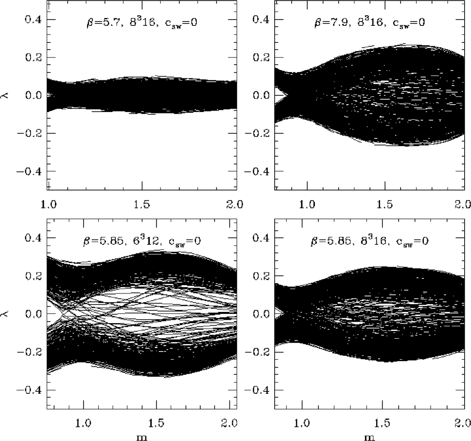
Figure 1: Spectral flow of the Wilson-Dirac ${\bf\rm H}_{L}(m)$ for the first four quenched ensembles in Table 1.

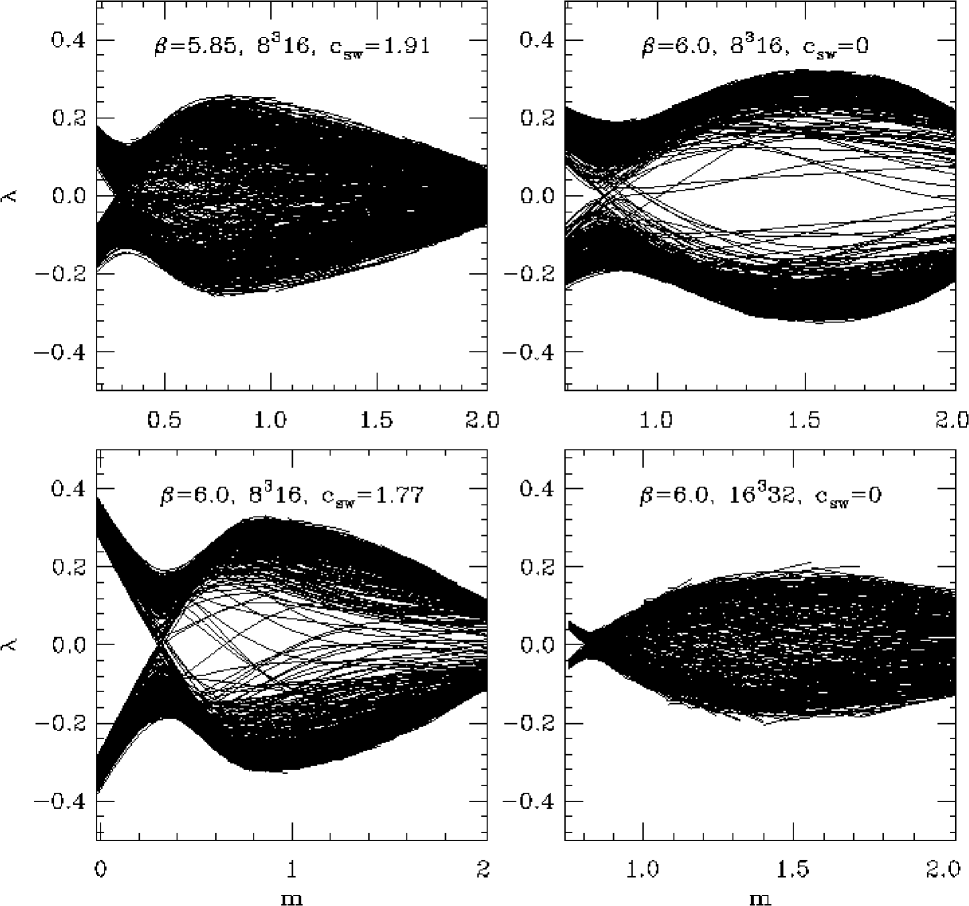
Figure 2: Spectral flow of the Wilson-Dirac ${\bf\rm H}_{L}(m)$ for the last four quenched ensembles in Table 1.

Figures 1 – 3 show the cumulative flow for the various ensembles in Table 1. Each figure is a cumulative plot of the spectral flow of the 10 lowest eigenvalues of ${\bf\rm H}^{2}_{L}(m)$ in one ensemble. Each figure shows a small region of $m$ where the gap is open – the end of region I as defined in the introduction. Most of each plot focuses on what was referred to as region II. This is the region where level crossings occur in the flow and where there are very low lying eigenvalues. The point in $m$ where the first crossing occurs in each ensemble is by definition the boundary, $m_{1}$, between regions I and II. The value of $m_{1}$ for the various ensembles is quoted in Table 2. We do not quote an error for this quantity since it is a number defined for the whole ensemble. The spectral flow for the ensemble of quenched $\beta=6.0$ configurations on the $8^{3}\times 16$ lattice using the SW improved ${\bf\rm H}_{L}(m)$ covers the entire region between $m=0$ and $m=2$ clearly showing region I where the gap is open.

As expected, $m_{1}$ decreases as we go to weaker coupling. It also decreases with the addition of an SW term to ${\bf\rm H}_{L}(m)$ due to the reduction of the additive renormalization of the mass term for improved Wilson fermions. One can compare $m_{1}$ with $m_{c}$ for the various ensembles, where $m_{c}$ is the “critical” mass where the pion mass computed in the region of positive physical quark mass extrapolates to zero. We note that where the data exists, this definition of $m_{c}$ agrees well with the PCAC determination of $m_{c}$ [15]. For the dynamical configurations, $m_{c}$ is defined using spectator Wilson quarks. We find $m_{c}>m_{1}$, indicating that $m_{c}$ lies inside region II. Increasing statistics, i.e. the number of configurations analyzed, can only decrease $m_{1}$.

We have plotted all the cumulative flows with the same scale on the y-axis to facilitate a comparison between the different ensembles. A comparison of the spectral flows of the unimproved ${\bf\rm H}_{L}(m)$ for $\beta=5.7,5.85$, and 6.0 on the $8^{3}\times 16$ lattice shows a thinning of the spectrum near zero for larger values of $m$ as one goes to larger values of $\beta$. In fact the gap seems to have essentially opened up for larger values of $m$ at $\beta=6.0$ on the $8^{3}\times 16$ lattice. However, we should keep in mind that the physical volume is getting smaller as one goes to higher values of $\beta$ at fixed lattice size. Two pairs of ensembles, (3) and (4) at $\beta=5.85$ and (6) and (8) at $\beta=6.0$, show us the effect of increasing the physical volume: the spectrum gets denser around zero for larger values of $m$ with increasing volume. Noting that in two pairs of ensembles, namely (1,8) at ($\beta=5.7$,$\beta=6.0$) and (3,6) at ($\beta=5.85,\beta=6.0$), the physical volume is essentially the same, we see that the spectrum gets thinner for a fixed physical volume as we go closer to the continuum limit.

A great deal of attention has recently been given to improved lattice actions. We therefore also studied the spectral flow of ${\bf\rm H}_{L}(m)$ on an ensemble, (2) in Table 1, of quenched configurations generated using the Symanzik improved gauge action [18] at a lattice gauge coupling of $\beta=7.9$ on an $8^{3}\times 16$ lattice. This ensemble has a lattice spacing in between those with Wilson action at $\beta=5.7$ and $5.85$ (see Table 2). The spectral flow looks very much like the one for the standard Wilson gauge action with the density in the large mass region in between that for the Wilson action ensembles at $\beta=5.7$ and $\beta=5.85$. Improving the gauge action seems to have little effect on the spectral flow. We also studied the effect of improving ${\bf\rm H}_{L}(m)$ by adding an SW term with the nonperturbatively determined SW coefficient of Ref. [15, 16]. We have done this for the quenched ensembles (5) and (7) on the $8^{3}\times 16$ lattices at $\beta=5.85$ and $6.0$. In accordance with the smaller additive mass renormalization we find that the gap closes at a smaller value $m_{1}$. The spectrum is denser around zero for larger values of $m$ and the effect of doubler modes seems to set in earlier – we attribute the decrease of the distance between the largest among the 10 lowest eigenvalues, as $m$ approaches 2, to the appearance of doubler modes. Like for the unimproved ${\bf\rm H}_{L}(m)$ the density around zero decreases as we go to the weaker coupling.

Finally we look at the effect of dynamical fermions on the spectral flow. We consider three ensembles with dynamical Wilson fermions and two ensembles with dynamical staggered fermions. All these ensembles have a lattice spacing that is roughly equivalent to a quenched Wilson action ensemble at $\beta=6.0$ (see Table 2). One should note that each of the dynamical ensembles has only 20 configurations. In contrast, all the quenched ensembles had 50 configurations, with the exception of the $\beta=6.0$ ensemble on a $16^{3}\times 32$ lattice which had 30 configurations. The spectral flows for all the dynamical configurations look more like the one for the $\beta=5.7$ quenched configurations indicating that the dynamical configurations behave as though they are on a coarser lattice than expected. This effect is more pronounced for the ensembles with dynamical Wilson fermions than for those with staggered quarks. We note that for the ensembles with dynamical Wilson fermions, as expected, the gap closes at a larger mass parameter $m_{1}$ than the $m_{d}$ of the dynamical fermions (recall that due to our sign convention a larger mass parameter corresponds to a smaller physical mass).

A measure of the density of eigenvalues at zero at a fixed value of $m$ can be obtained by considering the condensate as defined by

$$\rho(0;m)=\lim_{h\rightarrow 0}\lim_{V\rightarrow\infty}\rho_{h}(m)\qquad\rho_{h}(m)={1\over V}\langle\sum_{n}{h\over\lambda^{2}_{n}(m)+h^{2}}\rangle,$$ (2)

where $<\dots>$ indicates an average over a gauge field ensemble. In the thermodynamic limit indicated, $\rho(0;m)$ is the density of eigenvalues at zero (up to an irrelevant multiplicative factor). In this paper we approximate $\rho_{h}(m)$, at given fixed volume, by summing over the ten lowest eigenvalues and keeping $h$ fixed at $0.01$. When the gap is closed $\rho_{h}(m)$ of (2) is dominated by the lowest few eigenvalues. Our aim is to get a qualitative comparison of the dimensionless ratio $\rho_{h}(m)/\sigma^{3/2}$ for the various ensembles in Table 1 and to get a better understanding of the region where the gap is closed.

The various plots are shown in Figures 4 – 6. Comparing the plots for $\beta=5.7,5.85$ and $6.0$ on the $8^{3}\times 16$ lattice with no improvement term in ${\bf\rm H}_{L}(m)$, we see that a peak develops in the condensate close to the lower end of region II where the gap is closed. The peak becomes sharper as we go to weaker coupling and the condensate at larger values of $m$ becomes smaller. The addition of the SW term to ${\bf\rm H}_{L}(m)$ has the effect of raising the peak, but we do not see clear evidence for a sharpening of the peak. The suppression of the condensate at larger values of $m$, seen without the SW term, is now weakened. We see a rise in the condensate as $m$ is increased towards 2. This rise becomes smaller for weaker coupling albeit also in a smaller physical volume. We attribute this rise to an increased density of low eigenvalues due to doubler modes starting to become small.

Improving the gauge action ($\beta=7.9$ on an $8^{3}\times 16$ lattice) does not change the qualitative behavior of the condensate when compared to a standard Wilson action ensemble. However, the condensate for larger values of $m$ seem to be smaller than the condensate obtained using the standard Wilson action at $\beta=5.85$ even though the Symanzik improved ensemble is thought to be on a coarser lattice as seen comparing the values of the string tension in Table 2.

Turning now to the dynamical ensembles, we see a peak in the condensate and a slow rise for larger values of $m$. The peak seems to become somewhat sharper as one reduces the dynamical quark mass indicating a stronger signal for a condensate. The rise at larger mass parameter $m$ indicates that these configurations are farther away from the continuum limit than the quenched configurations at $\beta=6.0$, with the dynamical Wilson ensembles being farthest away.

3 Topology from level crossings

The net number of level crossings in ${\bf\rm H}_{L}(m)$ between $m=0$ and a fixed value $m_{t}<2$ results in a distribution of the index of the chiral Dirac operator at the chosen value $m_{t}$. Assuming that the index is the same as the topological charge of the gauge field background we can get an estimate for the topological susceptibility as a function of $m_{t}$. Naturally it can be non-zero only in region II since level crossings occur only in this region. By investigating the topological susceptibility as a function of $m_{t}$ we can get some understanding of the physical relevance of the crossings that occur at the larger values of $m$ where the condensate is small. The various plots are shown in Figures 7 – 9. All of them have the general characteristic that they show a sharp rise in the region where the condensate is peaked and then they essentially flatten out in the region where the condensate is small. This is the case also in the presence of the SW term, for the improved gauge action and for the ensembles that contain dynamical fermions. This presents convincing evidence that the level crossings that occur at larger $m$ are not physically relevant.

Further supporting evidence can be found by looking at the eigenvectors associated with level crossings. We find that all these eigenvectors are well localized on the lattice. To characterize the localization we use a definition of the size of the eigenvector inspired by the ’t Hooft zero mode and given in Ref. [8]. Other definitions motivated by an Anderson type localization can be found in [14]. However, since there is a natural connection between level crossings in ${\bf\rm H}_{L}(m)$ and topology, and since for smooth instanton backgrounds the shape of the eigenmode at a crossing point agrees very well with the ’t Hooft zero mode [3], we prefer the definition in Ref. [8]. We should emphasize that we look only at the sizes of eigenmodes that cross, and only close to the crossing point. Only then can we expect to get a good estimate of the localization size inspired by the ’t Hooft zero mode.

For each of the ensembles in Table 1, we have measured the sizes of all the modes that cross and we plot the localization size, in units of the lattice spacing, as a function of the crossing point $m$ in Figures 10 – 12. All plots show a monotonic decrease in the localization size as a function of the crossing point. There is a small deviation from the monotonic decrease at large $m$ for the flows obtained with an SW improvement term, probably due to the onset of crossings of doubler modes. The decrease of size is faster as one goes closer to the continuum limit. We can not see a significant change in the rate of decrease when we compare the plots with and without the SW term in ${\bf\rm H}_{L}(m)$. In all cases we see that the localization sizes associated with the level crossings in the region where the condensate is small are of the order of one to two lattice spacing. This shows that they are not physical, consistent with the finding that these crossings do not affect the topological susceptibility.

The estimate for the topological susceptibility from the flat region for the various ensembles, measured in units of the corresponding string tension, is listed in Table 2 and shown in Figure 13. The result for the quenched ensembles are plotted together as a function of $a^{2}\sigma$ to show the trend toward the continuum limit. There is no hard evidence for scaling yet though we do see that the results with and without the SW term agree. We note that the topological susceptibility at $\beta=5.85$ on the $6^{3}\times 12$ lattice and at $\beta=6.0$ on the $8^{3}\times 16$ lattice suffer from finite volume effects. For the dynamical ensembles, we plot the topological susceptibility as a function of $m^{2}_{\pi}/\sigma$, a measure of the physical quark mass. We note that the topological susceptibility measured using cooling on the two-flavor staggered ensembles [19] agree with the values here.

4 Consequences for domain wall fermions

Our study of the spectral flow of ${\bf\rm H}_{L}(m)$ has consequences to the study of vector gauge theories with massless quarks using domain wall fermions [7]. In the domain wall formalism with no explicit quark mass term, the fermion mass induced by the finite extent of the extra direction is exponentially suppressed for free fermions [7] and in one-loop perturbation theory [20]. Analytical studies pertaining to the domain wall formalism in the limit of an infinite extent in the extra direction can be found in Ref. [21].

The many body Hamiltonian for the propagation in the extra dimension in the domain wall formalism is $a^{\dagger}{\bf\rm H}_{D}(m)a$, where

$$e^{-{\bf\rm H}_{D}(m)}=T(m)=\pmatrix{{1\over 1-m+{\bf\rm B}}&{1\over 1-m+{\bf\rm B}}{\bf\rm C}\cr{\bf\rm C}^{\dagger}{1\over 1-m+{\bf\rm B}}&{\bf\rm C}^{\dagger}{1\over 1-m+{\bf\rm B}}{\bf\rm C}+1-m+{\bf\rm B}\cr}$$ (3)

is the transfer matrix for propagation in the fifth direction with the domain wall mass set to $m$ [1, 22]. In order to have an exponential suppression in the fifth direction in all physical observables, ${\bf\rm H}_{D}(m)$ should have a gap. The extent of the fifth direction, $L_{s}$, has to be chosen proportional to the inverse of the gap in ${\bf\rm H}_{D}(m)$ to suppress dependence on the extent of the fifth direction [22]. Zero eigenvalues of ${\bf\rm H}_{L}(m)$ studied in this paper are in one to one correspondence with zero eigenvalues of ${\bf\rm H}_{D}(m)$ [1]. In addition, the slope of the flow at the crossing point is the same [1]. Therefore the spectrum of ${\bf\rm H}_{D}(m)$ in the neighborhood of zero will be the same as the spectrum of ${\bf\rm H}_{L}(m)$. In particular, if ${\bf\rm H}_{L}(m)$ does not have a gap in some region of $m$, then ${\bf\rm H}_{D}(m)$ also will not have a gap in the same region of $m$. Then the ground state of $a^{\dagger}{\bf\rm H}_{D}(m)a$ is not separated from the first excited state by a gap and the dependence of observables on the extent of the extra direction will not be exponentially suppressed. This could apply, for example, to the fermion mass induced by the finite extent, $L_{s}$. We remark that the zero modes of ${\bf\rm H}_{D}(m)$ that are relevant for the discussion here do not correspond to zero modes of the five dimensional domain wall Dirac operator.

For the domain wall fermions to feel the effect of the gauge field topology, the domain wall mass must be larger than $m_{1}$. Our analysis shows that the gap does not open up again, and therefore there is no choice for the domain wall mass that leads to an exponential suppression. This fact is indepenent of the shape and sizes of the low lying modes. We would like to emphasize that the number of modes near zero increases with the volume as demonstrated by the condensate in Figures 4 and 5. The actual magnitude of the contamination from the excited states, on the other hand, will depend on the operator studied in the domain wall formalism, size and shape of the low lying modes of ${\bf\rm H}_{D}(m)$ and the spectral density of ${\bf\rm H}_{D}(m)$ near zero.

Domain wall fermions have been studied numerically on four dimensional quenched ensembles [23, 24]. However, these studies included an explicit non-zero positive quark mass, $m_{q}$. Effects of this explicit quark mass can be understood by looking at the fermionic determinant in an external gauge field background at finite extent $L_{s}$, given by [22]

$$\det\Bigl{[}{1+m_{q}+(1-m_{q})\gamma_{5}\tanh({1\over 2}L_{s}{\bf\rm H}_{D})\over 2}\Bigr{]}$$ (4)

where $m_{q}\leq 1$. Deviation of $\tanh({1\over 2}L_{s}{\bf\rm H}_{D})$ from $\epsilon({\bf\rm H}_{D})$ gives an additional, induced mass. If ${\bf\rm H}_{D}$ has a gap, this induced mass is exponentially suppressed, and to keep it at a constant fraction of $m_{q}$ would require only an increase of $L_{s}$ logarithmic in $m_{q}$, as $m_{q}$ is decreased. If there is no gap, the induced mass decreases only as some power of $1/L_{s}$ and $L_{s}$ has to be increased as some (fractional) power of $1/m_{q}$.

Evidence in support of the need to increase $L_{s}$ with decreasing $m_{q}$ exists in the data for the pion mass measured as a function of quark mass at $\beta=5.85$ in Ref. [25]. With a quark mass of $m_{q}=0.075$ they find that it is sufficient to have fourteen slices in the extra direction. But this is not sufficient at $m_{q}=0.05$ where the result from eighteen slices in the extra direction significantly deviates from the result obtained with fourteen slices. However, the results are not detailed enough to distinguish between the need of only a logarithmic increase in $m_{q}$, or a faster one, as we predict due to the absence of a gap. We find that the gap also remains closed at $\beta=6.0$ on an $16^{3}\times 32$ lattice and here again we predict the need of a faster than logarithmic increase of $L_{s}$ with decreasing $m_{q}$.

We have seen some evidence that the gap gets thinner for a fixed physical volume as one goes closer to the continuum. This is based on a comparison of the $\beta=5.7$ ensemble on the $8^{3}\times 16$ lattice with the $\beta=6.0$ ensemble on the $16^{3}\times 32$ lattice and a comparison of the $\beta=5.85$ ensemble on the $6^{3}\times 12$ lattice with the $\beta=6.0$ ensemble on the $8^{3}\times 16$ lattice. It is therefore conceivable that there exists a large enough physical volume where one does not expect any finite volume effects and a weak enough lattice coupling where the gap is essentially open, or at least the density of zero eigenvalues is small enough that one can use domain wall fermions efficiently to investigate massless QCD on the lattice. Based on our results, we predict that one needs $\beta>6.0$ if one wants to work with a short extent in the extra direction and be able to deal with very small explicit quark masses.

We have previously argued that the crossings occurring at larger $m$, where the density of low lying eigenvalues, and hence the condensate, is small, are unphysical. They do not affect the topological susceptibility and the localization size of the crossing modes are only of the order of one to two lattice spacing. It is these crossings, however, which hinder the use of domain wall fermions to study vector gauge theories. These crossings are generic and cannot be eliminated by any improvement of the Wilson-Dirac operator ${\bf\rm H}_{L}(m)$. This claim is based on the following heuristic argument: ${\bf\rm H}_{L}(m)$ has the structure of Eq. (1), with ${\bf\rm C}$ a discretization of the continuum chiral Dirac operator with all improvements and ${\bf\rm B}$ the Wilson term, again with all improvements. As argued in Ref [1] the non-commutativity of ${\bf\rm B}$ and ${\bf\rm C}$ is an essential feature of the generic Wilson-Dirac operator on the lattice that enables it to correctly describe a single physical particle and also correctly encode the topological content of the background gauge field. The operators ${\bf\rm B}$ and ${\bf\rm C}$ are bounded on the lattice and therefore the spectra of ${\bf\rm H}_{L}(m)$ at $m=\pm\infty$ are identical and contain an equal number of positive and negative eigenvalues. Therefore all crossings that occur in ${\bf\rm H}_{L}(m)$ have to occur in pairs. Due to the presence of the Wilson term ${\bf\rm B}$, crossings due to the unphysical particles (the doubler modes) do not occur in the neighborhood of $m=0$. In the continuum limit and for arbitrary smooth configurations, we expect crossings near $m=0$ due to the topological content of the background gauge field. Then we expect crossings in the opposite direction due to doubler modes near $m=2$. This has been verified for smooth SU(2) instanton backgrounds [3]. There it was also shown that the crossing point moved farther away from $m=0$ as the instanton size was decreased and the gauge configuration on the lattice thus became rougher. Not surprisingly an instanton with a size of the order of one lattice spacing crossed farthest away from zero. For instantons below a certain size (about one lattice spacing) no crossings were found. Since the crossing near $m=0$ is associated with an opposite crossing near $m=2$ due to the doubler, and since the flow changes continuously as we reduce the size of the background instanton, the two crossing points have to move closer together before they coincide, with the flow being tangent, and then disappear. This picture has to remain true for any ${\bf\rm H}_{L}(m)$ that conforms to the structure of Eq. (1). Therefore crossings will occur for any value of $m$ in the region $m_{1}\leq m\leq 2$. Since the action of the (small) instanton configurations is finite, they will be generically present in a lattice ensemble. But, all crossings beyond a small range close to the first crossing at $m_{1}$ are due to small localized modes and correspond to fluctuations on the scale of the ultraviolet cutoff.

Since the level crossings that occur for large values of $m$ in region II are due to localized modes of the order of one lattice spacing it is conceivable that these zero crossings can be “lifted”. We now describe one such modification to the domain wall formalism. The modified many body Hamiltonian describing the propagation in the extra direction has the following form:

$$\pmatrix{a^{\dagger}&b^{\dagger}\cr}\pmatrix{{\bf\rm H}_{L}(m)&m_{f}+{\bf\rm B}-m_{1}\cr m_{f}+{\bf\rm B}-m_{1}&-{\bf\rm H}_{L}(m)}\pmatrix{a\cr b\cr}$$ (5)

The diagonal entries describe the propagation of the left and right handed massless fermions. Here, $m_{f}$ is the bare fermion mass that couples the left and right handed fermions. The operator ${\bf\rm B}$ is the usual Wilson term also present in ${\bf\rm H}_{L}(m)$ but is now used to “lift” the zero crossings that occur away from $m_{1}$ in region II. In the absence of the off diagonal terms, the spectral flow is a superposition of the flow of $+{\bf\rm H}_{L}(m)$ and $-{\bf\rm H}_{L}(m)$. With $m_{f}=0$, ${\bf\rm B}-m_{1}$ will be small for crossings that occur close to $m_{1}$, namely the physical crossings. As such the pair of crossings that occur near $m_{1}$ will not be affected much and the low lying eigenvalues will remain low. However, the crossings far away from $m_{1}$ in region II will result in a large value for ${\bf\rm B}-m_{1}$ and will be lifted up. The spectral flow will have low lying eigenvalues around $m_{1}$ and will essentially have a gap beyond $m_{1}$. The addition of ${\bf\rm B}-m_{1}$ results in a mass term and the massless limit will no longer occur at $m_{f}=0$ away from the continuum limit. In spite of this, the above modification might be useful in practice to study domain wall fermions at reasonable gauge couplings without having to take $L_{s}$ to infinity as $m_{f}$ goes to zero.

5 Conclusions

We studied the spectral flow of ${\bf\rm H}_{L}(m)$ on several lattice gauge field ensembles with and without the presence of an SW term in ${\bf\rm H}_{L}(m)$. We found the value $m_{1}$, $0\leq m_{1}<2$, where the gap of ${\bf\rm H}_{L}(m)$ closes. In the large volume limit the gap remains closed for all values $m>m_{1}$, all the way up to $m=2$. We find $m_{1}$ decreases when going closer to the continuum limit and also when adding an SW improvement term to ${\bf\rm H}_{L}(m)$. In all cases we found that $m_{1}<m_{c}$ where $m_{c}$ is the point where the pion mass measured at values $m<m_{1}$ extrapolates to zero. A careful analysis of the spectral flow using a measure for the condensate showed that it exhibits a peak in region II where the gap is closed. The peak occurred at a value very close to $m_{1}$. The peak became sharper as one went to weaker coupling; however, we did not see any significant evidence for a sharpening of the peak upon the addition of the SW term. The presence of an SW term resulted in a rise in the condensate for large $m$ and so did the presence of dynamical fermions. The topological susceptibility measured using the net level crossing in ${\bf\rm H}_{L}(m)$ showed a sharp rise at the beginning of region II and then it remained quite flat for large $m$ where the condensate was small. By studying the size of the eigenmodes that cross we found that the levels that cross at larger $m$ correspond to modes that have a localization size of the order of one lattice spacing.

Improving the gauge action had no dramatic effect on the spectral flow. The condensate in the large $m$ region showed a slightly less pronounced rise than the corresponding Wilson gauge results at $\beta=5.85$ and $5.70$. Some effects of improvement did appear in the localization size distribution. In particular, the density of small modes appears reduced using the improved gauge action while the large modes near $m_{1}$ appear unaffected. Both results are within our expectations from the behavior of the condensate and the action improvement program.

The spectral flow on a variety of quenched ensembles has shown that the gap does not open after it has closed at a value of $m=m_{1}$. This hinders the use of domain wall fermions in quenched QCD. A modification of the domain wall fermions to overcome this problem has been proposed. One could also study dynamical domain wall fermions or use them as spectator fermions in dynamical ensembles generated using Wilson or staggered fermions. Our study of the flow in this paper shows that $\beta=5.5$ with dynamical Wilson fermions and $\beta=5.6$ with dynamical staggered fermions is not suitable for a study using domain wall fermions. It is necessary to go to weaker couplings when dynamical fermions are present. Our study of the flow of ${\bf\rm H}_{L}(m)$ has shown that an addition of an SW term to ${\bf\rm H}_{L}(m)$ does not help the situation for domain wall fermions. In fact, it seems to worsen. On the other hand it is probably not appropriate to include an SW term in ${\bf\rm H}_{L}(m)$ in the context of the domain wall formalism since domain wall fermions with a Wilson-Dirac Hamiltonian are already expected to be an improvement over Wilson fermions [20, 24, 25]. A study of the spectral flow at weaker couplings than the ones studied in this paper should help answer the question of the feasibility of domain wall fermions. In ensembles with dynamical Wilson fermions, only the gap for the dynamical fermion mass is really relevant for spectroscopy. In all the cases we studied in this paper, the spectrum has a gap at the dynamical fermion mass, that is to say that all these correspond to positive physical quark mass. It would be interesting to study the spectrum on dynamical ensembles generated with an unphysical quark mass. There will be a technical obstacle to this study on large volumes but a small volume study might be feasible.

Table 1: Description of ensembles analyzed in this paper.

Ensemble	Lattice size	Spectral	Flow	Number of
Type		parameters	parameters	configurations
1) Pure gauge	$8^{3}\times 16$	$\beta=5.7$	$c_{sw}=0$	50
Wilson [8]			$1<m<2$
2) Symanzik	$8^{3}\times 16$	$\beta=7.9$	$c_{sw}=0$	50
Improved			$0.8<m<2$
3) Pure gauge	$6^{3}\times 12$	$\beta=5.85$	$c_{sw}=0$	50
Wilson			$0.8<m<2$
4) Pure gauge	$8^{3}\times 16$	$\beta=5.85$	$c_{sw}=0$	50
Wilson			$0.84<m<2$
5) Pure gauge	$8^{3}\times 16$	$\beta=5.85$	$c_{sw}=1.91~{}\cite[cite]{[\@@bibref{}{scri}{}{}]}$	50
Wilson			$0.2<m<2$
6) Pure gauge	$8^{3}\times 16$	$\beta=6.0$	$c_{sw}=0$	50
Wilson			$0.7<m<2$
7) Pure gauge	$8^{3}\times 16$	$\beta=6.0$	$c_{sw}=1.77~{}\cite[cite]{[\@@bibref{}{alpha,scri}{}{}]}$	50
Wilson			$0<m<2$
8) Pure gauge	$16^{3}\times 32$	$\beta=6.0$	$c_{sw}=0$	30
Wilson			$0.76<m<2$
9) Two flavor	$16^{3}\times 32$	$\beta=5.5$	$c_{sw}=0$	20
Wilson [26]		$m_{d}=0.8672$	$0.88<m<2$
10) Two flavor	$16^{3}\times 32$	$\beta=5.5$	$c_{sw}=0$	20
Wilson [26]		$m_{d}=0.875$	$0.88<m<2$
11) Two flavor	$16^{3}\times 32$	$\beta=5.5$	$c_{sw}=0$	20
Wilson [26]		$m_{d}=0.8828$	$0.88<m<2$
12) Two flavored	$16^{3}\times 32$	$\beta=5.6$	$c_{sw}=0$	20
Staggered [27]		$m_{d}=0.025$	$0.84<m<2$
13) Two flavored	$16^{3}\times 32$	$\beta=5.6$	$c_{sw}=0$	20
Staggered [27]		$m_{d}=0.01$	$0.84<m<2$

Table 2: A listing of $m_{1}$ where the gap closes and the topological susceptibility for the various ensembles in Table 1

Ensemble	$a\sqrt{\sigma}$	$m_{c}$	$m_{1}$	$\chi^{1/4}/\sqrt{\sigma}$
1	0.392 [28]	1.047 [31]	1.025 [8]	0.44(2)
2	0.352 [29]	0.891 [29]	0.862	0.40(2)
3	0.286 [28]	0.908 [31]	0.857	0.35(3)
4	0.286 [28]	0.908 [31]	0.873	0.46(2)
5	0.286 [28]	0.283 [16]	0.267	0.47(2)
6	0.220 [28]	0.820 [31]	0.818	0.35(2)
7	0.220 [28]	0.302 [15]	0.297	0.37(2)
8	0.220 [28]	0.820 [31]	0.805	0.41(3)
9	0.254 [26]	0.929 [26]	0.914	0.54(4)
10	0.241 [26]	0.922 [26]	0.907	0.47(4)
11	0.226 [26]	0.914 [26]	0.904	0.37(2)
12	0.240 [30]	0.900 [32]	0.893	0.38(4)
13	0.219 [30]	0.894 [32]	0.880	0.41(3)

Figure 3: Spectral flow of the Wilson-Dirac ${\bf\rm H}_{L}(m)$ for four of the dynamical ensembles in Table 1.

Figure 4: A measure of the condensate for first of four quenched ensembles in Table 1.

Figure 5: A measure of the condensate for the last four quenched ensembles in Table 1.

Figure 6: A measure of the condensate for four of the dynamical ensembles in Table 1.

Figure 7: Topological susceptibility as a function of $m$ for the first four quenched ensembles in Table 1.

Figure 8: Topological susceptibility as a function of $m$ for the last four quenched ensembles in Table 1.

Figure 9: Topological susceptibility as a function of $m$ for four of the dynamical ensembles in Table 1.

Figure 10: Localization size of crossing mode in lattice units as a function of the crossing point for the first four quenched ensembles in Table 1.

Figure 11: Localization size of crossing mode in lattice units as a function of the crossing point for the last four quenched ensembles in Table 1.

Figure 12: Localization size of crossing mode in lattice units as a function of the crossing point for four of the dynamical ensembles in Table 1.

Figure 13: Plots of the topological susceptibility for the eight quenched ensembles and the five dynamical ensembles as a function of the string tension.

References

- [1] R. Narayanan and H. Neuberger, Nucl. Phys. B443 (1995) 305.
- [2] R. Narayanan and H. Neuberger, Phys. Rev. Lett. 71 (1993) 3251.
- [3] R.G. Edwards, U.M. Heller and R. Narayanan, hep-lat/9801015, To appear in Nuclear Physics B.
- [4] Y. Kikukawa, R. Narayanan and H. Neuberger, Phys.Rev. D57 (1998) 1233.
- [5] H. Neuberger, Phys. Lett. B417 (1998) 141.
- [6] D.B. Kaplan, Phys. Lett. B288 (1992) 342.
- [7] D.B. Kaplan, Nucl. Phys. Proc. Suppl. B30 (1993) 597; Y. Shamir, Nucl. Phys. B406 (1993) 90.
- [8] R.G. Edwards, U.M. Heller, R. Narayanan and R.L. Singleton, Jr., Nucl. Phys. B518 (1998) 319.
- [9] R. Narayanan and P. Vranas, Nucl. Phys. B506 (1997) 373.
- [10] R. Narayanan, H. Neuberger and P. Vranas, Phys. Lett. B353 (1995) 507.
- [11] P. Vranas, Phys. Rev. D57 (1998) 1415; Nucl. Phys. Proc. Suppl. B63 (1998) 603.
- [12] S. Itoh, Y. Iwasaki, T. Yoshie, Phys. Rev. D36 (1987) 527; W. Bardeen, A. Duncan, E. Eichten, G. Hockney and H. Thacker, Phys. Rev. D57 (1998) 1633; Nucl. Phys. Proc. Suppl. B63 (1998) 141; C.R. Gattringer, I. Hip and C.B. Lang, Nucl. Phys. B508 (1997) 329; C.R. Gattringer and I. Hip, hep-lat/9712015; P. Hernandez, hep-lat/9801035.
- [13] K. Jansen, Nucl. Phys. Proc. Suppl. B53 (1997) 127.
- [14] K. Jansen, C. Liu, H. Simma and D. Smith, Nucl. Phys. Proc. Suppl. B53 (1997) 262; D. Smith, H. Simma and M. Teper, Nucl. Phys. Proc. Suppl. B63 (1998) 558; H. Simma and D. Smith, hep-lat/9801025
- [15] M. Lüscher, S. Sint, R. Sommer, P. Weisz and U. Wolff, Nucl. Phys. B491 (1997) 323;
- [16] R.G. Edwards, U.M. Heller and T.R. Klassen, Phys. Rev. Lett. 80 (1998) 3448; in preparation.
- [17] B. Bunk, K. Jansen, M. Lüscher and H. Simma, DESY-Report (September 1994); T. Kalkreuter and H. Simma,Comput. Phys. Commun. 93 (1996) 33.
- [18] M. Lüscher and P. Weisz, Comm. Math. Phys. 97 (1985) 59; Phys. Lett. 158B (1985) 250; M. Alford, W. Dimm, G.P. Lepage, G. Hockney and P.B. Mackenzie, Phys. Lett. B361 (1995) 87;
- [19] K.M. Bitar, R. Edwards, S. Gottlieb, U.M. Heller, A.D. Kennedy, S. Kim, J.B. Kogut, A. Krasnitz, W. Liu, M.C. Ogilvie, R.L. Renken, D.K. Sinclair, R.L. Sugar, M. Teper, D. Toussaint, and K.C. Wang, Nucl. Phys. B30 (Proc. Suppl.) (1993) 315.
- [20] Y. Kikukawa, H. Neuberger and A. Yamada, hep-lat/9712022.
- [21] V. Furman and Y. Shamir, Nucl. Phys. B439 (1995) 54; S. Aoki and Y. Taniguchi, hep-lat/9711004; Nucl. Phys. Proc. Suppl. 63 (1998) 290.
- [22] H. Neuberger, Phys. Rev. D57 (1998) 5417.
- [23] T. Blum and A. Soni, Phys. Rev. D56 (1997) 174; Nucl. Phys. Proc. Suppl. 63 (1998) 287.
- [24] T. Blum and A. Soni, Phys. Rev. Lett. 79 (1997) 3595.
- [25] T. Blum and A. Soni, hep-lat/9712004.
- [26] K.M. Bitar, R.G. Edwards, U.M. Heller and A.D. Kennedy, Nucl. Phys. Proc. Suppl. B53 (1997) 225; in preparation.
- [27] K.M. Bitar et al. (HEMCGC Collaboration), Nucl. Phys. Proc. Suppl. B20 (1991) 362; Nucl. Phys. Proc. Suppl. B26 (1992) 259; Phys. Rev. D49 (1994) 6026.
- [28] R.G. Edwards, U.M. Heller and T.R. Klassen, Nucl. Phys. B517 (1998) 377.
- [29] S. Collins, R.G. Edwards, U.M. Heller and J. Sloan, Nucl. Phys. Proc. Suppl. B53 (1997) 877.
- [30] U.M. Heller, K.M. Bitar, R.G. Edwards and A.D. Kennedy, Phys. Lett. B335 (1994) 71.
- [31] M. Göckeler, R. Horsley, H. Perlt, P. Rakow, G. Schierholz, A. Schiller and P. Stephenson, Phys. Rev. D57 (1998) 5562.
- [32] K.M. Bitar et al. (HEMCGC Collaboration), Phys. Rev. D46 (1992) 2169; Phys. Rev. D48 (1993) 370.