LTH-420

hep-lat/9802015

February 10, 1998

Maximal variance reduction for stochastic propagators with applications to the static quark spectrum

UKQCD Collaboration

C. Michael and J. Peisa

Department of Mathematical Sciences, University of Liverpool,
Liverpool L69 3BX, UK

Abstract

We study a new method – maximal variance reduction – for reducing the variance of stochastic estimators for quark propagators. We find that while this method is comparable to usual iterative inversion for light-light mesons, a considerable improvement is achieved for systems containing at least one infinitely heavy quark. Such systems are needed for heavy quark effective theory. As an illustration of the effectiveness of the method we present results for the masses of the ground state and excited states of $\bar{Q}q$ mesons and $\bar{Q}qq$ baryons. We compare these results with the experimental spectra involving $b$ quarks.

1 Introduction

When computing hadron-hadron correlators, one needs quark propagators from a given source to a sink. Optimally one would like to calculate the propagators required from all sites to all sites, and thus use all information available from the finite number of gauge samples. In practice this is seldom possible as one has to invert the Wilson-Dirac fermion matrix to obtain the propagators. Using conventional iterative methods, one obtains propagators from one source to all given sinks; to calculate and store such propagators from all sources is virtually impossible with current computing resources. Furthermore there is no known way to stop iterating before one reaches the machine precision without introducing bias. Therefore one obtains extremely accurate propagators from few sources. The propagators are so accurate that the variance coming from the limited sample of gauge configurations dominates the results totally. Clearly a lot of time is wasted on calculating the propagators to such precision, when the variance from one gauge configuration to another is several orders of magnitude larger.

One possibility is to calculate also the propagators by Monte Carlo methods [1, 2, 3]. This allows one to store the propagators from everywhere to everywhere in a sensible amount of storage space and also avoids the unnecessary calculation of the propagators to machine precision.

It is easy to express the inverse of a positive definite matrix $A$ in a form suitable for Monte Carlo integration: one just takes a Gaussian integral

$$A_{ij}^{-1}={1\over Z}\int D\phi\,\phi_{j}^{*}\phi_{i}\exp(-{1\over 2}\phi^{*}A\phi),$$ (1.1)

which then can be treated exactly as a free scalar field on the lattice. If the matrix $A$ is local, it is easy to implement efficient Monte Carlo update techniques for the scalar field $\phi$, allowing one to calculate the required inverse of $A$. Thus, for a given gauge field, one would obtain $N$ independent samples of the $\phi$ fields by Monte Carlo and so evaluate the stochastic estimate of the required element of the inverse of $A$ by an average over these $N$ samples: $A_{ij}=\langle\phi_{j}^{*}\phi_{i}\rangle$. By storing these $N$ samples of $\phi$, one would then be able to evaluate propagators from any site to any site.

This is not directly applicable to the Wilson-Dirac fermion matrix $Q=1-\kappa M$, because $Q$ is not positive definite for those values of hopping parameter $\kappa$ that one is usually interested in. To obtain the propagators by the above method, one has to work with $A=Q^{\dagger}Q$, which is guaranteed to be positive definite. As $Q$ contains only nearest neighbour interactions, $A$ is still local – it contains at most next-to-nearest neighbour interactions, and an effective updating scheme can be implemented. Of course to recover the inverse of $Q$ instead of $A^{-1}$ one should modify eq. (1.1) to

$$G_{ji}=Q_{ji}^{-1}=\left<(Q_{ik}\phi_{k})^{*}\phi_{j}\right>,$$ (1.2)

which can then be used to calculate the propagators one needs for hadronic observables.

In practice a direct application of eq. (1.2) has a serious drawback when used in realistic lattice QCD calculations. Because the $\phi$ fields have a variance of order one coming from the gaussian distribution which determines them, the standard deviation on the estimate of the propagator will be of order $N_{s}^{-1/2}$ for $N_{s}$ samples of $\phi$ fields. Usually one is interested in the large $T$ behaviour of the correlators of hadronic observables. These correlators decay exponentially, and therefore the signal is exponentially small (like $\exp(-mT)$ where $m$ is the hadron mass) in the regime of interest. As the variance of the propagators calculated from eq. (1.2) is the same no matter how far in time they extend, it would be necessary to use impractical amounts of computer time to increase the number of samples $N_{s}$ sufficiently to obtain a reasonable signal to noise ratio at large $T$.

In this paper we will discuss stochastic methods to calculate propagators. We will compare several suggestions to avoid the problems described above, and show that it is possible to construct propagators from scalar fields that have their variance maximally reduced. We also discuss the use of improved fermionic actions with stochastic estimators.

To test different methods, we focus our attention to systems which contain one infinitely heavy quark as obtained in leading order heavy quark effective theory[4]. Such a study is appropriate in particular to the B meson and its excited states which are made of one heavy quark and one light quark. These systems are particularly problematic for conventional methods of evaluating light quark propagators, because, using one source for the light quark propagator, there will be only one measurement of the hadronic correlator to time $T$ per gauge configuration when the heavy quark is treated as static. Therefore it seems that one would benefit hugely from having propagators from all sources available. This benefit will then help to offset the extra noise coming from having only a stochastic estimate.

For mesonic correlations, the signal is linear in the light quark propagator and so no problems arise with biases or correlations among stochastic samples. A more careful analysis is needed for observables involving more than one light quark propagator. Here we study one example in detail: the baryonic system made of one static quark and two light quarks.

We also study the feasibility of applying our method of choice – maximal variance reduction – to systems where all the quarks are propagating.

2 Variance reduction

The method described in the previous section has a scalar field $\phi$ for which each component (fixing space-time, colour and Dirac index) has a typical variance of order 1. Thus the propagator will have a standard deviation of order $N_{s}^{-1/2}$ for $N_{s}$ samples of the $\phi$ fields. The most promising way to improve on this situation is to improve on the operator $\phi^{*}\phi$ used to calculate the stochastic estimators of $G_{ij}$ in eq. (1.1). Here we study in detail two different methods and discuss their advantages and suitability for effective implementation.

2.1 Local multihit

The easiest way to construct an operator that has a substantial reduction in variance is to observe that is it possible to perform a local multihit for the scalar fields $\phi$ needed for $G_{ij}$. This is analogous to the method proposed in [5] for pure gauge systems and is equivalent to performing an average over infinitely many samples of the chosen component of $\phi$ with all other components held fixed. This has been proposed in ref.[1] and clearly leads to a variance reduction. Because of the simple quadratic nature of the integration over $\phi$, the multihit average is obtained explicitly by

$$\phi_{i}\to-A_{ii}^{-1}A_{ij}\phi_{j}$$ (2.1)

with $i\neq j$ and no summation on $i$ and where, for the Wilson-Dirac case, the diagonal term is given by $A_{ii}=1+16\kappa^{2}$. Thus each $\phi$ field can be replaced by its multihit average. It is permissible to use these multi-hit values in place of $\phi$ in evaluating propagators and observables involving products of $\phi$ fields provided that no $\phi$ field is in the neighbourhood of another — that is no pair of $\phi$ fields can be linked by $A$ and so are not nearest or L-shaped next-to-nearest neighbours. This multihit improvement is easily implemented with only a minimal effect on the computer time consumption and it provides a marked improvement over no variance reduction. This improvement is independent of the extent $T$ of the fermion propagation, however. Thus though the improvement is substantial, it does not allow a study of large $T$. This is because the method only averages over the nearest and next-to-nearest neighbours of each site, thus taking into account only local variations in the scalar fields.

2.2 Maximal variance reduction

Instead of averaging over only near neighbours of a given site, one could use all fields inside some given region $R$. Let $s_{i}$ be the scalar field variables at the boundary of $R$ and consider submatrices of the matrix $A$: firstly $\tilde{A}$ containing elements that link the $\phi$ fields inside the region $R$ to those on the boundary and secondly $\bar{A}$ containing only links between the fields totally inside the region $R$. Now to average simultaneously over all scalar fields inside $R$ while keeping the fields $s_{i}$ on the boundary fixed, it is sufficient to replace $\phi$ at a given site $i$ with the average obtained from the following expression:

$$v_{i}={1\over\cal{Z}}\int D\phi\,\phi_{i}\exp\,-{1\over 2}\left(\phi^{*}_{j}\bar{A}_{jk}\phi_{k}+\phi_{j}^{*}\tilde{A}_{jk}s_{k}+s_{j}^{*}\tilde{A}_{jk}\phi_{k}\right).$$ (2.2)

Because the integral (2.2) is gaussian, one can easily calculate it analytically to obtain

$$v_{i}=-\bar{A}^{-1}_{ij}\tilde{A}_{jk}s_{k}.$$ (2.3)

where $i,\ j\in R$ and $k\not\in R$. We will call $v$ the variance reduced estimator for $\phi$. By combining two such improved estimators, each from disjoint regions $R$ and $R^{\prime}$ respectively, one obtains a variance reduced estimator for propagator $G$ from any point in $R$ to any point in $R^{\prime}$. The choice of the two regions $R$ and $R^{\prime}$ is arbitrary (subject to the constraint that the two regions should not overlap in the sense of being linked by $A$). The local multihit described above corresponds to taking each region as just one site. However, we can now optimise the choice of regions to obtain maximal variance reduction.

In order to calculate $v$ in given gauge configuration, one needs the inverse of $\bar{A}$ from an extended source – the scalar field $s_{i}$ at the boundary of $R$. This is computationally equivalent to a single inversion of the Dirac-Wilson fermion matrix in region $R$. If the volume of $R$ is large, this is computationally demanding and so the method is not immediately advantageous. The gain comes from the fact that once this inversion is done, one can efficiently evaluate the propagators from every site inside region $R$ to every site inside region $R^{\prime}$. If the cost of calculating the necessary scalar configurations is not too high, one should gain a substantial amount of CPU time compared to conventional methods. In addition the reduction in variance should be much greater than for the local multihit method, as one averages the $\phi$ fields over a larger region. In the case of fairly heavy quarks, one can estimate analytically the variance reduction using the hopping parameter expansion: this gives a reduction of $\kappa^{d}$ where $d$ is the minimum number of links from the boundary of $R$ to the interior point under consideration, and likewise for $R^{\prime}$. Thus it is feasible that a stochastic evaluation of a hadronic correlator involving a separation of $T$ time steps will have its variance reduced by $\kappa^{T}$. This achieves our goal of evaluating efficiently large time propagators.

In a sense, both local multihit and maximal variance reduction are three level Monte Carlo updating algorithms:

1. One generates gauge configurations $g$ with a suitable algorithm.

2. In each $g$ one generates stochastic samples $\phi$ according to distribution in eq. (1.1).

3. For each scalar field configuration one generates improved operators keeping some of the original fields $\phi$ fixed. This can be done analytically (or with Monte Carlo) for both maximal variance reduction and local multihit.

Since the last step can be performed analytically by an iterative scheme, the computational effort involves one inversion per stochastic sample. Thus for $N_{s}$ stochastic samples per gauge field, one will have to perform roughly $N_{s}/12$ inversions compared to conventional extraction of the propagator from all colour-spins at one source point. However, one gets access to the propagator from all sources to all sinks which may more than compensate. We now explore the implementation.

3 Implementation

To compare different methods, we have implemented the stochastic inversion method, both with local multihit and with maximal variance reduction.

If one is using unimproved Wilson fermions, writing the Monte Carlo algorithm for scalar fields is straightforward. The only complication arises from the fact that the action contains next-to-nearest-neighbour interactions. To be able to vectorize our algorithm in the style of the conventional red-black partition of odd and even sites, we assigned the lattice sites to 32 “colours” and updated each colour sequentially. For parallel machines such a partitioning is unnecessary. The actual heat bath and overrelaxation algorithms are simple. The local action, obtained directly from eq. (1.1) by keeping only terms involving $\phi_{x}$ with others fixed, is just

$$S_{loc}={1\over 2}\left(\phi_{x}^{\dagger}C\phi_{x}+\phi_{x}^{\dagger}a_{x}+a_{x}^{\dagger}\phi_{x}\right),$$ (3.1)

with $C=1+16\kappa^{2}$ and

$$a_{x}=-\kappa M_{xi}^{\dagger}\phi_{i}-\kappa M_{xi}\phi_{i}+\kappa^{2}M_{xi}^{\dagger}M_{ij}\phi_{j},$$ (3.2)

where one should note that all sums over sites exclude the $x$-site. Completing the square, then

$$S_{loc}={1\over 2}\left(\phi_{x}+{a_{x}\over C}\right)^{\dagger}C\left(\phi_{x}+{a_{x}\over C}\right),$$ (3.3)

and the heat bath algorithm is equivalent to generating gaussian random numbers with variance $C^{-1}$ and equating them to $\phi_{x}+a_{x}/C$. For the gaussian random numbers we use the Cray library function SLARNV. The overrelaxation is equally straightforward: one just flips

$$\phi_{x}\to\phi_{x}-{2a_{x}\over C}$$ (3.4)

for each Dirac and colour component of $\phi$.

In evaluating $a_{x}$, it is very inefficient to use the matrix $A$ directly since it connects 54 sites to $x$. As in eq. (3.2), using the result that $A=(1-\kappa M)^{\dagger}(1-\kappa M)$, it is preferable to work with $M$ directly since it only has an implicit sum over 8 sites. Then the main computational load in evaluating $a_{x}$ comes from the gauge part of the matrix multiplication $M\phi$. If one keeps $\psi=M\phi$ in memory as well as $\phi$ itself, then the evaluation of $a_{x}$ from $M^{\dagger}(-\kappa\phi+\kappa^{2}\psi)-\kappa\psi$ involves only one application of $M^{\dagger}$ to a vector. One then needs, however, to update $\psi$ which involves work equivalent to a further application of $M$ to a vector. This strategy reduces the total work needed to the equivalent of two applications of $M$ to a vector.

In practice we found that, after initialising using heatbath sweeps, it was efficient to use combined sweeps of 4 overrelaxation plus one heatbath to give sufficiently equilibrated and independent samples. We discuss the number of such sweeps in detail later. Where independence of the samples is at a premium, one can choose to combine only samples further apart - this we explored and we report later on the result. In general, as one approaches the chiral limit of light quarks, one expects the fermion matrix $A$ to have small eigenvalues with spatially extended eigenvectors. These will cause critical slowing down of our local updating scheme. Similar considerations apply to using bosonic algorithms for dynamical fermions [6] and multi-grid and other methods are known to be available to circumvent this problem in principle.

For the Sheikholeslami-Wohlert improved clover action [7] the algorithm is not much more complicated. The Dirac-Wilson fermion matrix $Q$ is replaced by

$$Q_{SW}=L-\kappa M\ ,$$ (3.5)

where $L$ is diagonal in space-time but not now in colour and spin and depends on the coefficient $c_{SW}$ which is 1.0 in lowest order perturbation theory and, as discussed later, can be estimated by tadpole improvement or non-perturbative improvement:

$$L=1-{c_{SW}\over 16}\kappa\sum_{\mu\nu}F^{\mu\nu}\sigma_{\mu\nu}\ ,$$ (3.6)

where $F_{\mu\nu}$ is defined here at each site as the lattice operator $\sum_{P}(U_{P}-U_{P}^{\dagger})$ given by the 4-leaved clover sum over plaquettes on the lattice in the $\mu,\ \nu$ plane where $U_{P}$ is the product of the four links around a plaquette $P$ and where

$$\sigma_{\mu\nu}={1\over 2}\left[\gamma_{\mu},\gamma_{\nu}\right]\ .$$ (3.7)

Note that $L$ is hermitian.

The local action is still quadratic in the $\phi$ field at a site $x$ as given by eq. 93.1), but $C$ is now a matrix in Dirac and colour indices:

$$C = \left(1-{c_{SW}\over 16}\kappa F^{\mu\nu}\sigma_{\mu\nu}\right)^{\dagger}\left(1-{c_{SW}\over 16}\kappa F^{\mu\nu}\sigma_{\mu\nu}\right)+16\kappa^{2},$$ (3.8)

$$a_{x} = -\kappa\left(1-{c_{SW}\over 16}\kappa F^{\mu\nu}\sigma_{\mu\nu}\right)^{\dagger}M_{xi}\phi_{i}-\kappa M_{xi}^{\dagger}\left(1-{c_{SW}\over 16}\kappa F^{\mu\nu}\sigma_{\mu\nu}\right)\phi_{i}$$ (3.9)

$$+\kappa^{2}M_{xi}^{\dagger}M_{ij}\phi_{j}\ .$$

For updating a given colour-spin component of $\phi$, we only need the inverse of the appropriate real diagonal element of $C$. However, the non-diagonal terms in $C$ need to be added to the force term $a_{x}$. With these changes, the actual updating algorithms for the clover action are the same as for unimproved Wilson fermions. As well as storing intermediate results ($M\phi$ and $L\phi$) to save computation as described for the Wilson case, the clover term can be treated efficiently by noting [8] that projecting $\phi=\phi_{+}+\phi_{-}$, where $\phi_{\pm}={1\over 2}(1\pm\gamma_{5})\phi$, allows $L$ and $C=L^{\dagger}L$ to be represented as two $6\times 6$ hermitian matrices rather than one $12\times 12$ matrix at each site.

In addition to Monte Carlo algorithms for scalar fields one needs an iterative inversion algorithm in region $R$ to implement the maximal variance reduction with source $\tilde{A}_{jk}s_{k}$. Since the matrix $\bar{A}$ is hermitian, a reliable method is conjugate gradient and this is what we use. Since the condition number of $A=Q^{\dagger}Q$ is considerably worse than that of $Q$ itself, it may well be faster to use a method such as minimal residual to invert the non-hermitian matrix $Q$ and then in turn to invert $Q^{\dagger}$, particularly if an efficient preconditioner such as red-black can be used for these inversions. Since the present study is exploratory, we have not investigated this option further. Another option is that since we need to invert $\bar{A}$ for the same gauge configuration with $N_{s}$ different sources $s_{k}$ coming from the stochastic Monte Carlo described above, inversion methods using multiple sources may offer some computational benefit.

We now discuss the optimum choice of the partitions $R$ and $R^{\prime}$ for applications. Sites in $R$ and $R^{\prime}$ must not be connected by $A$. The matrix $A$ contains nearest and next-to-nearest link terms. Because of the spin projection ${1\over 2}(1\pm\gamma_{\mu})$ contained in the $\pm\mu$ -directed link term of the Wilson fermion matrix $M$, $A$ does not contain any terms with double straight links. Thus a simple way to divide $R$ and $R^{\prime}$ is by a time-plane on which the sources $s_{k}$ lie. Since the lattice is periodic in time (or antiperiodic for fermions), the optimum situation is to have two such boundaries, for example at $t_{1}=0$ and $t_{2}=T/2$ where $T$ is the time extent of the lattice. Then any propagator from the region $0\leq t\leq T/2$ to the region $T/2\leq t\leq T$ can be evaluated. Note that propagators from one region to the source area $S$ are allowed and will be variance reduced. A propagator entirely within one region will involve two $\phi$ fields (say at $x$ and $y$) in that region and the integration over the fields inside $R$ of eq. (2.2) will then give an extra disconnected term involving $\bar{A}^{-1}_{xy}$. This is just a propagator within region $R$ and so we are back to the problem of evaluating it for all pairs of points $x$ and $y$ in $R$. Thus our present method does not allow any variance reduction for a propagator corresponding to a disconnected fermion loop.

In applications, we create $N_{s}$ independent samples of the scalar field $\phi(x)$ for each gauge configuration. We then use the $\phi$ field as a source on time planes $t_{1}$ and $t_{2}$ to obtain the variance reduced fields $v(x)$ for each sample in $R$ and $R^{\prime}$. As well as $v$ in $R$ and $R^{\prime}$, we then only need to store $\phi(x)$ on the two source time-planes (which we call region $S$). So each variance-reduced sample has storage of $24\times L^{3}\times T$ real numbers which is equivalent to one twelfth of the storage of the usual propagator from one point to all sinks. These variance reduced fields then allow improved estimators of the propagator from any point in $R+S$ to any point in $R^{\prime}+S$. This allows a determination of hadronic correlators involving one light quark using nearly all points as sources and sinks. We will investigate whether the increase in statistics from using so many source points is sufficient to compensate for the stochastic noise inherent in the method.

We now discuss the choice of the number of samples $N_{s}$. If too many samples were used, the determination of the correlator of interest might have a variance from one gauge configuration which is smaller than the variance over many gauge configurations. In other words, there will be no advantage in measuring too accurately on one gauge configuration. For correlators involving one light quark, the partition of computational effort between more samples $N_{s}$ per gauge or more gauge configurations is not crucial. Provided one does not overdo $N_{s}$ as describe above, the signal should be comparable for a given product of $N_{s}$ and number of gauge configurations.

When more than one light quark propagator is to be evaluated stochastically in an unbiased way, the considerations of optimum $N_{s}$ are more subtle. Provided the scalar field samples are independent, the two light quark propagators, each from $R+S$ to $R^{\prime}+S$, can be estimated from $N_{s}^{2}$ combinations of the samples on each gauge configuration (${1\over 2}N_{s}(N_{s}-1)$ combinations if both light quarks have the same mass so are taken from the same set of samples). This suggests that the noise on the combined signal may decrease as fast as $N_{s}^{-1}$ in this case. This would imply that larger values for $N_{s}$ were more efficient in this case. We will report on our investigation of this point.

For studies of baryons or of matrix elements involving mesons, three or more light quark propagators are needed. Provided no propagator lies entirely within one of the regions $R$ or $R^{\prime}$ this is feasible. For mesonic matrix elements, one way to achieve this is to put the matrix element insertion on the source time-plane ($S$).

4 Static systems

We have chosen the system containing one light and one infinitely heavy quark (static quark) as our main test case. This system describes the $B$ meson in leading order heavy quark effective theory. With conventional light quark inversion techniques, the propagator from one source only is evaluated and this allows the hadronic correlator to be obtained from only two sink locations on a given gauge configuration for a given $T$. This makes very little use of the information contained in the gauge field. In contrast, the stochastic approach allows the hadronic propagators to be determined from very many more sites. Furthermore since the hadronic observable is linear in the light quark propagator, any problems of correlations among the statistical samples of the $\phi$ fields are irrelevant. This is thus an optimum area for testing the stochastic method. Indeed previous work [1] using multi-hit improvement has already concentrated in this area. Here we compare our maximal variance reduction approach with this approach and also with the conventional iterative inversion. Our main point of comparison will be the B-meson correlation at $T=7$.

Because of the flexibility of the stochastic method, it is possible to study non-local hadronic operators with no additional computational effort. Since orbital excitations involve non-local operators, this allows a comprehensive study of the excited state spectrum of heavy-light mesons. This is an area where comparatively little is known, so we are able to show the power of our approach by determining several new features of the excited B meson spectrum. We also explore the baryonic spectrum in the static limit and report on the comparison with other lattice work and with experiment.

4.1 B meson in the static limit

Following the conventions of [9], we use nonlocal operators for the B meson and its excited states. This will enable us to study also the orbitally excited mesons - the details are collected in the Appendix. The operator $B$ we use to create such a $\bar{Q}q$ meson on the lattice is defined on a timeslice $t$ as

$$B_{t}=\sum_{x_{1},x_{2}}\bar{Q}_{(}{\bf x}_{2},t)P_{t}({\bf x}_{1},{\bf x}_{2})\Gamma\,q({\bf x}_{1},t)\ .$$ (4.1)

$Q$ and $q$ are the heavy and light quark fields respectively, the sums are over all space at a given time $t$, $P_{t}$ is a linear combination of products of gauge links $U$ at time $t$ along paths $P$ from ${\bf x}_{1}$ to ${\bf x}_{2}$, $\Gamma$ defines the spin structure of the operator. The Dirac spin indices and the colour indices are implicit. The masses are then calculated from the exponential fall off of the $B\bar{B}$ correlation function (or vacuum expectation value)

$$C(T) = \left<B_{t}\bar{B}_{t+T}\right>_{0}$$ (4.3)

$$= \left<\bar{Q}({\bf x}_{2},t)P_{t}({\bf x}_{1},{\bf x}_{2})\Gamma q({\bf x}_{1},t)\right.\times$$

$$\left.\bar{q}({\bf x}^{\prime}_{1},t+T)P_{t+T}({\bf x}^{\prime}_{1},{\bf x}^{\prime}_{2})\Gamma^{\dagger}Q({\bf x}^{\prime}_{2},t+T)\right>_{0}$$

$$= \mbox{Tr }\left<P_{t}\Gamma G_{q}({\bf x}^{\prime}_{1},t+T,{\bf x}_{1},t)P_{t+T}\Gamma^{\dagger}G_{Q}({\bf x}_{2},t,{\bf x}^{\prime}_{2},t+T)\right>_{0}\ .$$ (4.4)

We have denoted the light and heavy quark propagators by $G_{q}$ and $G_{Q}$ respectively and the trace is over Dirac and colour indices and also includes the spatial sums over ${\bf x}_{1}$, ${\bf x}^{\prime}_{1}$, ${\bf x}_{2}$ and ${\bf x}^{\prime}_{2}$. Because we work with static heavy quarks, up to an irrelevant overall constant, one has

$$G_{Q}({\bf x}_{2},t,{\bf x}^{\prime}_{2},t+T)={1\over 2}(1+\gamma_{4})U^{Q}({\bf x}_{2},t,T)\delta_{{\bf x}_{2},{\bf x}^{\prime}_{2}}\ ,$$ (4.5)

where the gauge link product for the heavy quark is

$$U^{Q}({\bf x},t,T)=\prod_{i=0}^{T-1}U_{4}({\bf x},t+i)\ .$$ (4.6)

Now for the light quarks, we wish to evaluate the propagator $G_{q}$ by stochastic methods using eq. (1.2) where now angle brackets refer to the average over the $N_{s}$ stochastic samples. An alternative form can be obtained for the Wilson-Dirac discretisation, for which $Q(x,y)=\gamma_{5}Q(y,x)^{*}\gamma_{5}$ where $x$ includes space-time, colour and spin labels. This is

$$G_{ji}=\gamma_{5}\langle(Q_{jk}\phi_{k})\phi_{i}^{*}\rangle\gamma_{5}\ .$$ (4.7)

In practice, we find it optimum to evaluate both of these expressions eq. (1.2) and eq. (4.7) using our stochastic estimators and average them. Since we shall need it frequently, we define $\psi_{i}=Q_{ij}\phi_{j}$.

Using eq. (4.5) for the heavy quark propagator and stochastic scalar fields according to eq. (1.2) for the light quark propagator in eq. (4.4) one gets

$$C(T)=\mbox{Tr }\left<P_{t}\Gamma\phi({\bf x}^{\prime}_{1},t+T)\psi^{*}({\bf x}_{1},t))P_{t+T}\Gamma^{\dagger}{1\over 2}(1+\gamma_{4})U^{Q}({\bf x}_{2},t,T)\right>\ .$$ (4.8)

By choosing different path combinations and appropriate choices of $\Gamma$ in eq. (4.1) one can obtain different $J^{P}$ states as described in the Appendix. For the ground state B mesons in the static limit, we will have a degenerate pseudoscalar and vector. (The splitting between them can be evaluated by taking matrix elements of the clover term $\sigma_{\mu\nu}F_{\mu\nu}$ in the B ground state). The simplest hadronic operator to create these states is then obtained from eq. (4.1) by choosing $P_{t}=1$ and $\Gamma=\gamma_{5}$ for the pseudoscalar and $\Gamma=\gamma_{i}$ for the vector. From eq. (4.8) one obtains

$$C(t)={\rm Tr}\ H_{-}\ \left<\phi(x)U^{Q}({\bf x},x_{4},t)\psi^{*}(x+\hat{4}t)\right>\ ,$$ (4.9)

where $H_{\pm}=(1\pm\gamma_{4})/2$. The sum over Dirac indices is very simple with our convention in which $\gamma_{4}$ is diagonal and, making the colour sums explicit too, this is

$$C(t)=\sum_{x}\sum_{i=3,4}\left<\phi_{ai}(x)U^{Q}_{ab}({\bf x},x_{4},t)\psi_{bi}^{*}(x+\hat{4}t)\right>\ .$$ (4.10)

The alternate expression (4.7) for the stochastic light quark propagator yields

$$C(t)=\sum_{x}\sum_{i=1,2}\left<\psi_{ai}(x)U^{Q}_{ab}({\bf x},x_{4},t)\phi_{bi}^{*}(x+\hat{4}t)\right>\ .$$ (4.11)

If we now want to use maximally variance reduced operators instead of $\phi$ and $\psi$, one has to pay attention to the fact that $\phi$ and $\psi$ must not come from the same partition. Here we choose the simplest partition with sources at time planes $t_{1}$ and $t_{2}$. One subtlety is that $\psi=Q\phi$ is smeared out by one link in each direction: thus $\psi(t_{1})\phi(t_{1}+t)^{*}$ with $t>0$ would be invalid. Our favoured setup (which we tested to have minimal variance and which corresponds naively to taking the estimators as far as possible from the source) is to take $\psi$ at $t_{1}\pm(t/2)_{+}$ and $\phi$ at $t_{1}\mp(t/2)_{-}$ where if $t$ is odd $(t/2)_{+}$ is rounded up, etc. So for $t=1$ we have $\psi(t_{1}\pm 1)\phi(t_{1})^{*}$. Since the drop-off of $\phi$ from the source at $t_{1}$ is roughly exponential up to half way between the source time-slices, other partitions of $t$ have variance which is not much greater than our favoured setup. The complication is how to combine efficiently several estimators which have somewhat different variance.

To improve the overlap of our operators with the ground state, we have also considered fuzzed operators. These have paths $P_{t}$ formed by joining the light and heavy quarks by straight links of length $l$ in all 6 spatial directions. These links are themselves spatially fuzzed [10] using an iterative scheme. We use two different lengths $l$ each with a different number of fuzzing iterations as well as the unfuzzed operators described previously. Correlations of all combinations at each end are evaluated giving us a $2\times 2$ or $3\times 3$ matrix.

4.2 Comparison of methods

Since there is a considerable body of data on B meson correlations for Wilson fermions, we first tested our approach with Wilson fermions.

For comparison purposes, we considered a small lattice ($8^{3}$ 16) at $\beta=5.74$ with Wilson fermions of hopping parameter $K=0.156$. This choice was motivated by pre-existing studies [11]. As a first example we evaluated the B meson correlator at time separation $t$ using local hadronic operators at source and sink. Then we compared conventional inversion with various implementations of stochastic inversion. Results for the correlator $C(7)$ at $t=7$ are shown in Table 1 where the comparison has been made for equal disk storage of propagators or scalar field samples.

For the stochastic inversion methods we used 20 gauge configurations, each containing 25 samples of the scalar field. For the gauge fields we use 100 combined sweeps of one Cabibbo-Marinari pseudo-heatbath algorithm followed by 3 overrelaxation steps between configurations. The scalar fields were evaluated as described previously by using 125 heatbath plus overrelaxation updates between measurements after 250 sweeps to thermalise the first sample for each gauge configuration. We tested that our results were unchanged if more thermalisation sweeps were used. For the conventional MR inversion method we used 4 different sources on 10 gauge configurations. Since the storage of the conventional propagator from one source involves 12 colour-spins, it is the same as the storage of 12 stochastic scalar fields, so the comparison is made at equal file storage.

Table 1: B meson correlators at $t=7$.

Method	$C(7)\times 10^{7}$	Data Set	CPU
MR inversion	3712(147)	propagators from 4 sources	1
		for 10 gauge fields
Stochastic inversion		25 samples of $\phi$
Basic	2754(926)	for 20 gauge fields	2
Local multihit	3418(410)		2
Maximal variance reduction	3761(21)		4

Figure 1: The B meson effective mass versus $t$ from our data at $\beta=5.74$ from $8^{3}\times 16$ lattices with Wilson fermions and different combinations of local, fuzzed and $\gamma_{i}D_{i}$ sources and sinks together with a three exponential fit. Also shown (squares) are the Wuppertal data [11] for smeared source and local sink from 170 propagators.

Clearly the maximal variance reduction gives a factor of 7 improvement in error for only an overall computational increase of a factor of 4. This is equivalent to a net gain of a factor of 12 in computing time for a similar result. Moreover, the stochastic method allows correlations involving different sources (smeared, fuzzed, orbitally excited, etc) to be constructed at little extra cost. This is shown in fig. 1 where a comparison is made of our results for the effective mass with results [11] from conventional inversions (with 170 propagators) which are seen to be significantly less precise than those obtained here in the $t$ region of interest. More details of the fit are presented in ref. [2].

In order to explore more fully the power of the method of maximal variance reduction of stochastic propagators, we then undertook a more extensive study using clover improved fermions. In this case the focus of attention was on the precise determination of the B meson spectrum and excited states.

4.3 The excited B meson spectrum

Our results are not only useful for comparing different methods but are also physically interesting in their own right. In particular, the spectrum of the exited states in the static limit has not been thoroughly studied and experimental information on this spectrum is also limited. Moreover, without a precise extraction of the excited state component in the S-wave, the ground state contribution will be uncertain which implies systematic errors in extracting heavy-light matrix elements (for example $f_{B}$).

In order to study these new areas of physics using the power of stochastic inversion with maximal variance reduction, we determine the spectrum of heavy-light mesons and their excited states in the static limit. In order to minimise order $a$ effects, while still keeping in contact with existing simulations, we have used a tadpole improved action at $\beta=5.7$. A non-perturbatively improved [12] action is preferable to the tadpole-improved prescription on theoretical grounds but the determination of the appropriate value of the clover coefficient $c_{SW}$ has not been feasible for $\beta\leq 6.0$. The results at larger $\beta$ than 5.7 do, however, suggest that the non-perturbative value for $c_{SW}$ would be significantly larger than the tadpole value we use here. We also wish to keep finite size effects under control so we use two spatial lattice sizes.

We have performed simulations on $8^{3}\times 16$ and $12^{3}\times 24$ lattices with $\beta=5.7$ with $c_{SW}=1.57$ and we study two different values of hopping parameter: $\kappa_{1}=0.14077$ and $\kappa_{2}=0.13843$. These values have been used before to study the effect of tadpole improvement on the light meson spectrum [13] and pseudoscalar meson and vector meson masses are available from that work (see also Table 5). The chosen light quark masses correspond roughly to the strange quark mass ($\kappa_{1}$) and to twice the strange quark mass ($\kappa_{2}$). We will describe our light quark masses in dimensional units by quoting $(r_{0}m_{P})^{2}$ where $r_{0}/a=2.94$ is used at $\beta=5.7$ from our own interpolation. A recent independent study [14] gave $r_{0}/a=2.99(3)$ at this $\beta$ value. We also use $r_{0}$ to set the scale of the B meson masses. In terms of conventional units, $r_{0}\approx 0.5$ fm.

For the 20 pure gauge configurations we use a conventional scheme with 200 combined sweeps of 3 overrelaxation plus one heatbath between configurations. We evaluate $N_{s}=24$ scalar field samples per gauge configuration using 25 combined sweeps of 4 overrelaxation plus one heatbath, after 125 heatbath sweeps to initialise from a cold start. In each case we then evaluate the variationally improved scalar fields using conjugate gradient in the regions between time slices 0 and $T/2$. For the hadronic operators we use spatial fuzzed links which are iteratively evaluated [10] by summing ($f\times$ straight + sum of 4 spatial U-bends) and projecting the result to SU(3). Using $f=2.5$, we choose two fuzzed superlinks: (i) 2 iterations of fuzzing with superlinks of length 1, and (ii) 8 iterations of fuzzing with superlinks of length 2. When we explore Bethe Saltpeter wavefunctions for B mesons, we also employ other lengths for superlinks.

Our basic method for extracting the mass spectrum is to fit the matrix of zero-momentum correlators at a range of time separations to a factorising sum of several states. We use either two states or three, and in the latter case we may fix the mass of the third state to 2.0 in lattice units to stabilise the fit. A typical effective mass plot can be seen in Figure 2, where we have plotted the effective mass of the $L=0$ (S) state together with a factorising fit. We use either uncorrelated fits or some model of the correlation [15]. Typically the modelled correlation (this is the correlation among measurements from different gauge samples) is used to find the $t$ range giving acceptable fits. Then an uncorrelated fit is used to give the central values of the masses and other parameters. Statistical errors are determined by bootstrap of the gauge configurations. The systematic errors from fitting are estimated by varying the fit range in $t$ and the fit correlation model - these systematic errors are only quoted if they are significantly larger than the statistical errors.

Figure 2: Effective mass plot for the $S$-wave $\bar{Q}s$ meson using clover fermions on $12^{3}\times 24$ lattice at $\beta=5.7$ with light quark hopping parameter $\kappa_{1}=0.14077$.

Table 2: B meson effective masses.

state	$\kappa$	L	$am$	$am^{\prime}$	$\chi^{2}$/dof	$t$ range
S	1	12	0.875(06)	1.271(10)	32/54-11	4-12
P-	1	12	1.214(43)	1.727(53)	28/60-11	3-12
P-	1	12	1.194(48)	1.697(54)	13/30-8	3-12
P+	1	12	1.262(56)	1.698(57)	20/30-8	3-12
D±	1	12	1.555(12)	1.825(35)	22/27-6	4-12
D-	1	12	1.423(20)	1.751(27)	41/30-6	3-12
D+	1	12	1.744(56)	2.039(61)	15/30-6	3-12
F±	1	12	1.850(36)	2.053(44)	28/30-6	3-12
S	1	8	0.877(26)	1.273(44)	17/30-11	4-8
P-	1	8	1.200(90)	1.647(73)	12/18-8	3-8
P+	1	8	1.222(120)	1.774(70)	20/15-8	3-7
S	2	12	0.912(06)	1.284(10)	35/54-11	4-12
P-	2	12	1.313(17)	1.797(32)	77/60-11	3-12
P-	2	12	1.329(19)	1.809(41)	41/30-8	3-12
P+	2	12	1.386(27)	1.823(24)	21/30-8	3-12
D±	2	12	1.578(10)	1.826(30)	38/21-6	3-10
D-	2	12	1.480(13)	1.773(18)	34/30-6	3-12
D+	2	12	1.710(43)	1.883(45)	28/30-6	3-12
F±	2	12	1.901(24)	2.102(54)	53/30-6	3-12
S	2	8	0.899(12)	1.290(21)	11/30-11	4-8
P-	2	8	1.263(50)	1.837(48)	12/18-8	3-8
P+	2	8	1.224(71)	1.721(49)	5/18-8	3-8

Our results for the masses are collected in Table 2.

Here the different operators used correspond to those defined in the Appendix. The two values quoted for the $P_{-}$ state correspond to (i) using the same fit as for the $P_{+}$ state to yield the mass difference most reliably and (ii) using the extra operators available for the $P_{-}$ case to get the best mass determination. We determined the mass difference of the $P_{-}$ and $P_{+}$ using a bootstrap analysis of this difference and obtain, from the $12^{3}$ spatial lattices, values of the mass difference in lattice units of 0.068(64) at $\kappa_{1}$. The $P_{+}$ state for strange light quarks is thus heavier than $P_{-}$ with a significance of 1 standard deviation. For the D-wave states, we find for the mixed operator (labelled $D_{\pm}$) a mass consistent with lying between the masses of the two states separately. The splitting between the $D_{-}$ and $D_{+}$ masses appears to be quite large

The absolute values of the masses obtained in the static limit are not physical because of the self-energy of the static quark. We present masses by taking the difference with the ground state S-wave state (the usual B meson). The dependence on the orbital angular momentum is shown in Fig. 3 for strange quarks ($\kappa_{1}$). This suggests that the energy of the orbital excitations is linear with angular momentum.

The dependence on the light quark mass (through $\kappa$) would be expected to be small since the effect should be similar for each state and so cancel in the difference. Our results from the larger lattice are broadly compatible with this picture - see Fig. 4 where our results from $\kappa_{1}$ and $\kappa_{2}$ are plotted.

Figure 3: The masses of excited $Q\bar{s}$ mesons versus angular momentum $L$ from clover fermions with $\kappa=0.14077$. For the $L=2,\ 3$ states, results from operators which are a mixture of the two levels are also plotted. The straight line is to guide the eye. The scale is set by $a(5.7)=0.91$GeV^-1.

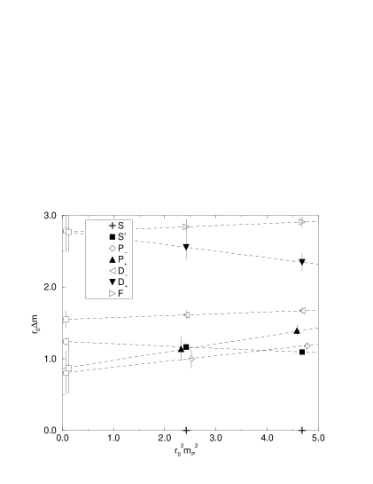
Figure 4: The spectrum of B mesons containing one light (with mass proportional to pseudoscalar mass $m_{P}^{2}$) and one infinitely heavy quark. Masses are given in terms of $r_{0}$. The straight lines show a linear chiral extrapolation.

We see evidence of significant finite size effects in comparing our results at $L=8$ and $L=12$. Because of this, we do not show results in Table 2 from our smaller spatial lattice for the higher lying excitations where the effect of the finite spatial size could be even larger. One specific example of the finite size effects is that, for $\kappa_{2}$, the $P_{+}$ state appears lighter than $P_{-}$ for $L=8$ while the order is the other way around at $L=12$, although the statistical significance of these level orderings is limited. This order of the $P_{\pm}$ levels at $L=8$ was also found in our results [2] from Wilson fermions. This is an issue of direct physical interest since potential models indicate that the long range spin-orbit interaction can, in principle, yield a $P_{+}$ state lying lighter than the $P_{-}$ as the light quark mass decreases to zero. Our larger volume results do not support this scenario and we find the $P_{-}$ state to lie lower than $P_{+}$ with a significance of 1 $\sigma$. To explore this in more detail, we need to establish the effect of the finite size effects. This is especially relevant for excited states, since they would be expected to be more extended spatially. This can be studied by determining the wavefunctions of the various states.

We can determine the Bethe Saltpeter wave functions $w(R)$ of the B meson states directly by fitting the ground state contribution (of the form $w(R_{1})w(R_{2})\exp(-mt)$) to a hadronic correlator where the operators at sink and source are of spatial size $R_{1}$ and $R_{2}$ respectively. Thus we measure correlations for a range of spatial extents $R$ of the lattice operators used to create and destroy the meson. We explore this at our larger lattice volume. In practice, following [10], we use straight fuzzed superlinks of length $R$ (we keep the number of iterations of fuzzing fixed at 4 here). After fitting, we extract the wavefunctions which are plotted for light quark mass corresponding to $\kappa_{2}$ in Fig. 5. This clearly shows the expected behaviour of higher orbital excitations being more spatially extended. Moreover, it shows evidence that the $P_{+}$ state is fatter than the $P_{-}$ which could explain the mass difference dependence on volume noted above - namely that the $P_{+}$ state has a modified mass at $L=8$. Changing the light quark mass from $\kappa_{2}$ to $\kappa_{1}$ results in no change in the wavefunctions within errors.

Another comforting conclusion is that there is evidence that the excited S-wave state has a node at radius $R\approx 1.5a$ which corresponds to $0.5r_{0}$. This implies that the meson has a nodal surface with a diameter of approximately $r_{0}$ which is broadly compatible with the result [10] for S-wave mesons made from two light quarks that the node for the excited state occurs at a diameter of about $6a$ at $\beta=6.0$ which again corresponds to $r_{0}$.

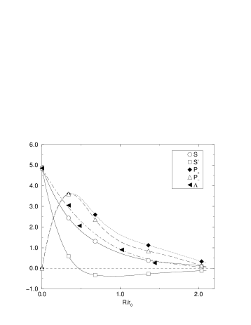
Figure 5: The Bethe Saltpeter wave function of the $\bar{Q}q$ mesonic states. The radius $R$ of the light quark $q$ from the static quark $Q$ is given in units of $r_{0}$. Here the light quark mass corresponds to $\kappa_{2}$. For the $\Lambda_{b}$ baryon, the results shown are obtained as described in the text. The continuous lines are to guide the eye.

We should like to explore also the lattice spacing dependence of our results since, even with an improved fermionic action, some residual discretisation effects are expected at $\beta=5.7$. We chose as parameters $\beta=5.9$ with $c_{SW}=1.5$ and $\kappa_{2}=0.1375$ with a $12^{3}\times 24$ lattice. Here we expect $r_{0}/a\approx 4.5$ which implies that the lattice spacing is 2/3 of that at $\beta=5.7$. Thus the spatial lattice size corresponds to $L=8$ at 5.7. This, unfortunately, means that the finite size effects on the excited states will still be significant, as found above. For this reason we do not pursue this study here, waiting instead until we have resources to enable us to study larger spatial sizes than $12^{3}$.

4.4 Baryons

In addition to mesons, we are also interested in $QL_{1}L_{2}$ baryons where $L_{i}$ refers to a $u,d$ or $s$ quark and $Q$ is a static quark. Since $b$ quarks are close to static, we describe such states by that name. We only consider states with no orbital angular momentum here, so in the static limit these baryonic states can be described by giving the light quark spin and parity. The lightest such state is expected to be the $\Lambda_{b}$ baryon with light quarks of $S^{P}=0^{+}$ which can be created by the local operator with Dirac index $i$:

$$\epsilon_{abc}Q_{ia}u_{jb}(C\gamma_{5})_{jk}d_{kc}$$ (4.12)

We treat the two light quarks as different, even if they have the same mass on the lattice. Experimentally, these states will be the $\Lambda_{b}$ and $\Xi_{b}$ for $ud$ and $qs$ light quarks respectively, where $q$ means $u$ or $d$.

In the static limit for the $b$ quark, there will be only one other baryonic combination [16] with no orbital angular momentum, namely the $\Sigma_{b}$ and degenerate $\Sigma_{b}^{*}$ with light quarks of $S^{P}=1^{+}$ created by

$$\epsilon_{abc}Q_{ia}u_{jb}(C\gamma_{r})_{jk}d_{kc}$$ (4.13)

In this case we average over the three spatial components $r$. Experimentally these states will be the $\Sigma_{b}$, $\Sigma_{b}^{*}$, $\Xi_{b}^{\prime}$, $\Xi_{b}^{*}$, and $\Omega_{b}$, $\Omega_{b}^{*}$ for $qq$, $qs$ and $ss$ light quarks respectively.

There are some computational issues. As two light quarks are involved, we need to use different stochastic samples for each. These can be obtained variance improved fields $v$ in $R$ and $R^{\prime}$ but a little care is needed when both light quarks have the same mass. One way to grasp the subtlety is to imagine that there are two quarks with different flavours. Then one has to split the sum over samples $\alpha=1\ldots N_{s}$ into subsets for each flavour. If these subsets are independent, one obtains propagators of each flavour with no bias. In practice if the stochastic estimators $\phi^{\alpha}$ are independent of $\alpha$, one can calculate the required propagators from

$$G_{ji}^{\alpha}G_{j^{\prime}i^{\prime}}^{\beta}=\sum_{\alpha\neq\beta}(Q_{ik}v_{k}^{\alpha})^{*}(Q_{i^{\prime}k^{\prime}}v_{k^{\prime}}^{\beta})^{*}v_{j}^{\alpha}v_{j^{\prime}}^{\beta}.$$ (4.14)

where $k,\ k^{\prime}\in R$ and $j,\ j^{\prime}\in R^{\prime}$. The $\Lambda_{b}$ correlator is then easily constructed by multiplying two light quark propagators from eq. (4.14) by the gauge links corresponding to a heavy quark propagator with the appropriate $\gamma$ matrix contractions. Note that since we save the stochastic samples and their variance reduced fields, we need very little extra computation to study this area. In order to be sure that there is full independence of the $\alpha$ and $\beta$ samples we chose $|\alpha-\beta|>3$ with our stochastic Monte Carlo parameters described previously. This reduces the statistics very little while increasing the number of sweeps between samples.

Note that because approximately $N_{s}^{2}$ samples are used, the error on the stochastic method decreases faster with $N_{s}$ for baryons. This is illustrated in Fig. 6 for one gauge configuration. Here the local operators are used for S-wave B meson and $\Lambda_{b}$ respectively and the correlator from 1 gauge configuration at $t=7$ with $N_{s}$ stochastic samples of mass $\kappa_{2}$ is plotted with errors coming from a jackknife analysis.

Figure 6: Relative error as a function of the stochastic sample size $N_{s}$. For the S-wave B meson containing only one light quark the decrease is consistent with $N_{s}^{-1/2}$, while for the $\Lambda_{b}$ baryon the decrease is consistent with $N_{s}^{-1}$. The results are from one gauge configuration at $\beta=5.7$ with clover fermions at $\kappa=0.13843$ on a 12³ 24 lattice for the correlation of local hadronic operators at $t=7$.

For our study of the spectrum we use, as previously, $N_{s}=24$ from 20 gauge configurations. For each of the light quarks we use either a local coupling or a sum of straight fuzzed links of length $l=1$ where 2 iterations of our fuzzing were used. This gives three hadron operators (neither, one and both light quarks fuzzed) which we employ at source and sink. Using both available hopping parameters for the light quark gives the results shown in Table 3. Note that the results with mixed hopping parameters (labelled 12) have higher statistics since the full set of stochastic samples are used (i.e. $N_{s}^{2}$). The mass values in Table 3 come from 2 state fits to the matrix of correlators in the $t$ range shown. We chose $t_{\rm max}<12$ in the fit because the signal was too noisy at larger $t$.

The dependence of these baryon masses on the light quark content appears consistent with the mesonic results in Table 2 that the mass in lattice units is 0.037 heavier when a light quark with $\kappa_{2}$ replaces one with $\kappa_{1}$. The exception is that the result for $\Sigma_{b}$ with mixed hopping parameters seems anomalously light - this appears to be a statistical fluctuation caused by our limited number of gauge samples.

We may also explore the Bethe Saltpeter wavefunctions in a similar way as for the B mesons. The additional feature for these baryons is that there are two light quarks and so a definition of radius is not unambiguous. We use two types of operator, (i) with one light quark fuzzed by a superlink of radius $l$ and the other at 0, and (ii) with both light quarks at radius $l$. We then varied the fuzzing radius $l$ and extracted the ground state coupling. One feature is the same as that found for light baryons [10] - namely the distributions of the two cases are similar if the radius in the double fuzzed case is increased by a factor of $\sqrt{2}$ which is a simple way to take into account the mean squared radius of the three dimensional double fuzzed case. With this interpretation, some results for the $\Lambda_{b}$ are included in Fig. 5. We find a very similar distribution for the $\Sigma_{b}$.

We also evaluated the baryonic correlations on spatial lattices with $L=8$. They are similar to those found for $L=12$ but, because of the more limited statistics and time extent, it is difficult to extract a stable signal from the fit so we are unable to quantify the finite size effects on the mass.

Table 3: $\Lambda_{b}$ and $\Sigma_{b}$ effective masses.

Baryon	$t$-range	$\kappa$	$am$
$\Lambda_{b}$	4-9	11	1.435(37)
$\Sigma_{b}$	5-9	11	1.514(52)
$\Lambda_{b}$	4-9	12	1.476(35)
$\Sigma_{b}$	5-9	12	1.493(25)
$\Lambda_{b}$	4-9	22	1.514(31)
$\Sigma_{b}$	5-9	22	1.621(27)

4.5 Comparison with earlier results and experiments

Since we are using a quenched Wilson action at $\beta=5.7$, for quantities defined in terms of gauge links, there will be order $a^{2}$ effects in mass ratios from this discretisation. For the $0^{++}$ glueball, the dimensionless product with $r_{0}$ has been extensively studied and substantial order $a^{2}$ effects are observed [17]. Indeed this ratio at $\beta=5.7$ is only 65% of the continuum value. It is commonly thought that the $0^{++}$ glueball has especially large order $a^{2}$ effects, so that other quantities may well have smaller departures at $\beta=5.7$ from their continuum values.

Discretisation effects arising from the fermionic component are of order $a$ for a Wilson fermion action. A SW-clover improvement term reduces this and a full non-perturbative choice [12] of the coefficient $c_{SW}$ would remove this order $a$ discretisation error. As discussed above, at $\beta=5.7$, the non-perturbative improvement scheme can not be implemented because of exceptional configurations. A more heuristic tadpole-improvement scheme can give estimates in this region and that is what we have employed here. From a thorough study of the light quark spectrum in this scheme in ref.[13] with the parameters we use here, we can establish the region that we are exploring.

Because of the significant discretisation effects in the region of parameters we are using, a definitive study would require results at larger $\beta$ so that extrapolation to the continuum limit would be possible. In this exploratory study, we present results at the coarse lattice spacing to show the power of the stochastic inversion method in extracting signals for hadrons. Since the study of light quark hadrons at this lattice spacing [13] does show qualitatively the features of the continuum limit, we present our results in way that allows comparison with experimental data.

The extrapolation to the chiral limit is uncertain in the quenched approximation because of effects from exceptional configurations and because of possible chiral logs. Thus, as well as giving the chirally extrapolated results, we present our results without extrapolation to avoid that source of systematic error. This can be achieved by interpolating to the strange quark mass for the light quark. Following ref.[13], we define the strange quark mass by requiring $m_{V}(\bar{s}s)/m_{P}(\bar{s}s)=1.5$, and assuming that the quark mass is proportional to the squared pseudoscalar mass, which gives $\kappa_{1}$ as $0.91(2)m_{s}$ and $\kappa_{2}$ as $1.77(4)m_{s}$. Hence we can extract results for strange light quarks by interpolation (as 90% those with $\kappa_{1}$ and 10% those with $\kappa_{2}$).

Equating $m_{V}(\bar{s}s)$ to the $\phi$ meson gives the scale $a=0.82$ GeV^-1. This can be compared with the scale obtained from using $r_{0}$ (see below) which gives $a=0.91$ GeV^-1. The scale obtained from different observables is likely to be different because of the coarse lattice spacing, and indeed differences of order 10 % are seen in ref.[13] when comparing with known continuum results.

Another issue is the possibility of finite size effects. The study of the light quark spectrum [13] shows no sign of any significant difference going from spatial size $L=12$ to $L=16$. This encourages us to expect that some of our results for $L=12$ may be close to those for infinite spatial volume. We can check this by comparing with $L=8$ and by looking at the Bethe-Saltpeter wavefunctions for the different states, as discussed above.

We first compare our results, using $r_{0}/a(5.7)=2.94$, to lattice results obtained using usual inversion techniques. In Figure LABEL:figure:mBcomp(a,b) we have plotted results which several other groups [18, 19, 11] have obtained in the static limit using much more computing resources. Note that some of these earlier works [11, 18] only use un-improved Wilson fermions. Our results are clearly consistent with earlier lattice results, within the errors quoted. However, we have smaller error bars and are able to obtain reliably several excited states, which is not generally true for the earlier work in the static limit.

We also present, in Table 4 and in Figure LABEL:figure:mBcomp(c,d), our results in MeV by assuming that the scale is set by $r_{0}=2.68$ GeV^-1. To avoid self energy effects from the static quark, mass differences are evaluated and we choose as input the ground state S-wave B mesons with strange light quarks. In the heavy quark limit, this S-wave B meson should be identified with the centre of gravity of the pseudoscalar and vector B mesons. There will be an overall scale error which may be significant and is expected to be at least 20% on energy differences. We also provide results extrapolated to massless light quarks assuming that the B meson masses are linear in $m_{P}^{2}$ - where in the table $s$ and $q$ refer to strange light quarks and massless light quarks respectively. As discussed above there will be significant systematic errors from this chiral extrapolation if it is not purely linear, as well as the statistical errors from bootstrap shown in the table. The chiral extrapolation for higher lying states may also be effected by finite size effects too. A further issue is the residual effect in heavy quark effective theory from treating the $b$ quark as static - this has been estimated to be around 40 MeV for the $\Lambda_{b}-B$ mass difference [16] and around 30-50 MeV for the S-P splitting in B mesons [20] which gives an order of magnitude estimate of this source of error.

Table 4: Heavy-light Spectrum in MeV

State	$J^{P}$	latt($s$)	expt($s$)	latt($q$)	expt($q$)
$B(S)$	$0^{-}$, $1^{-}$	input	5404	5356(16)	5313
$B(S^{\prime})$	$0^{-}$, $1^{-}$	5835(12)	-	5819(40)	5859(15)
$B(P_{-})$	$0^{+}$, $1^{+}$	5784(50)	5853(15)	5655(113)	5778(14)
$B(P_{+})$	$1^{+}$, $2^{+}$	5838(50)	5853(15)	5679(130)	5778(14)
$B(D_{-})$	$1^{-}$, $2^{-}$	6001(25)	-	5934(43)	-
$B(D_{+})$	$2^{-}$, $3^{-}$	6349(60)	-	6392(120)	-
$B(F)$	$2^{+}$, $3^{+}$, $4^{+}$	6475(50)	-	6409(83)	-
$\Lambda_{b}$	${1\over 2}^{+}$	6023(41)	-	5921(89)	5641(50)
$\Sigma_{b}$	${1\over 2}^{+}$, ${3\over 2}^{+}$	6113(57)	-	5975(60)	5851(50)

Comparing our results, remembering that only the statistical errors are included in Table 4, with experiment [22, 21, 23], we see several discrepancies. Note, however, that some assignments of excited states experimentally are rather uncertain, for instance the excited strange B meson seen at 5853 MeV has no definite $J^{P}$.

One feature is that the dependence of the B meson mass on the light quark mass is smaller than experiment. To compare with different lattice groups, we evaluate the dimensionless quantity which is the slope of $m_{B}$ versus the squared light-quark pseudoscalar meson mass, where a common light quark is used in the heavy-light and light mesons,

$$J_{b}={1\over r_{0}}{dm_{B}\over dm_{P}^{2}}$$

From our two $\kappa$ values, we find $J_{b}=0.048(13)$. Previous lattice determinations in the static limit [18, 19, 24] show consistency with a linear dependence and give values of $J_{b}$ between 0.05 and 0.08. The results of ref.[18] with Wilson light quarks show some evidence for an increase of $J_{b}$ from $\beta=5.7$ to 6.1. The experimental value of the $B_{s}$ to $B_{d}$ mass difference is 90 MeV and, using the string tension ($\sqrt{K}=0.44$ GeV) to set the scale of $r_{0}$, gives $J_{b}=0.074$. The mass difference of $D_{s}$ to $D_{d}$, taking the centre of gravity of the vector and pseudoscalar states, is about 103 MeV and since the corrections to the HQET limit are expected to behave like $1/m_{Q}$, the change from the $b$ quark to static quarks should be very small for this quantity - of order 2%. In summary, our quenched lattice result for $J_{b}$ appears to be low compared to experiment - as also found by ref.[24].

This is reminiscent of the case for light quark mesons, where in the quenched approximation, a similar property is found - summarised [25] by the $J$ parameter (proportional to slope of $m_{V}$ versus $m_{P}^{2}$) which is typically 0.37 rather than the experimental value of 0.48(2). This is equivalent to ‘the strange quark problem’ of quenched QCD where a consistent way to set the strange quark mass is not possible. This seems to carry over, in our work, to the heavy-light spectrum. As well as in the $B$ spectrum as described above, we also see the same effect in the light quark mass dependence of the $\Lambda_{b}$ baryon - as discussed previously.

The spectrum of mesonic excited states can be compared with experimental data which has been interpreted as showing evidence for the assignments given [21, 22, 23]. Our result for the radial excitation appears to agree well while the P-wave results agree qualitatively too. We give our predictions for the higher orbital excitations too. The finite size effects on these excited states should be more significant than on the ground state and, thus, this source of systematic error may only be removed by exploring even larger spatial volumes than here.

Our results for $\Lambda_{b}$ are significantly larger than experiment. We have checked that there do not appear to be significant systematic errors from extracting the ground state signal. Our results for the baryonic correlations from $8^{3}$ spatial lattices do not suggest any very strong finite size effects either. Moreover, as seen in Fig. 4, we agree with other lattice determinations in the static limit although the statistical significance of these earlier studies is quite low. The discrepancy in conclusion compared with ref.[19] is in the extrapolation to the chiral limit. The lattice results agree within errors but the slope of the $\Lambda_{b}$ mass versus $m_{P}^{2}$ is rather different which leads to the much lower mass value in the chiral limit from ref.[19].

As well as lattice results in the static limit, studies have been undertaken with propagating quarks. The conventional method implies a significant extrapolation in heavy quark mass to reach the $b$ quark - and even more so to compare with static quarks. More relevant to our work is the NRQCD method which allows heavy quarks to be used explicitly on a lattice. This NRQCD method has also been used to study this area and has reported [20] preliminary mass values for $b\bar{q}$ S and P-wave mesons and for $bqq$ baryons with light and strange quarks in qualitative agreement with experiment. Their results suggest a level ordering with the $P_{+}$ state above the $P_{-}$ by about 200 MeV with a significance of $4\sigma$. Their results for the baryonic levels are lower than ours, in better agreement with experiment.

5 Non-static systems

The simplest such situation is the spectrum of mesons made from 2 light quarks. To test our approach, we have compared the results from stochastic maximal variance reduction with conventional methods [13].

As a cross check, we have measured pseudoscalar and vector meson masses for clover fermions on 12³ 24 lattices at the same parameters as ref.[13]. We use superlinks of length $l=3$ made from links with 5 fuzzing iterations as well as local observables and a two state fit with the excited state fixed at $am=1.75$ to stabilise the fit. We obtain from $N_{s}=24$ samples on 20 gauge configurations the results shown in Table 5. The values from conventional inversions on 500 gauge configurations [13] clearly have much smaller errors than our method using 20 gauge configurations. By increasing our sample size $N_{s}$, we could improve our signal/CPU, since the noise decreases as $1/N_{s}$, but the conventional method works very well here. In principle, one gains by increasing $N_{s}$ only until the noise from finite sample size is comparably small to the inherent fluctuations from gauge configuration to gauge configuration. This limit on $N_{s}$ will depend on the observable under study and other parameters and, after exploring values of $N_{s}$ up to 96, we find that in general it is greater than 96.

The main reason that the stochastic maximal variance reduction is so noisy is that our variance reduction is in terms of the number of links (in the time direction) from the source planes. The zero-momentum meson correlator involves a sum over the whole of the source and sink time-planes. The noise from each term in this sum is similar even though the signal is small at large spatial separation differences. Thus we get noise from the whole spatial volume whereas the signal is predominantly from a part of the volume. This same problem also plagues large spatial volume studies of glueballs and the solution [26] in that case is to evaluate the non-zero momentum correlators since they are related to the well measured part at relatively small spatial separation. This approach should help equally with our stochastic maximal variance reduction method.

Table 5: Pseudoscalar and Vector meson masses

Meson	$\kappa$	$t$-range	$am$	ref.[13]
$P$	11	3-12	0.523(30)	0.529(2)
$V$	11	3-12	0.731(87)	0.815(5)
$P$	22	3-12	0.740(36)	0.736(2)
$V$	22	3-12	0.977(48)	0.938(3)

Even though the meson mass spectrum is rather noisy compared to conventional inversions, there is a substantial gain from using our all-to-all techniques when exploring matrix elements of mesons. In this case three or more light quark propagators will be needed and they must be from more than one source point. This is straightforward to evaluate using our stochastic techniques with our stored sample fields. We intend to explore this area more completely elsewhere.

One of the problems, in the quenched approximation, with the conventional approach to light quark propagators is that exceptional configurations cause huge fluctuations in the correlation of hadrons, especially of pions, at hopping parameters close to the chiral limit. These exceptional configuration problems are associated with regions of non-zero topological charge. Using all-to-all propagators may smoothen these fluctuations somewhat in that the average over the spatial volume will fluctuate less than the propagator from one site. Eventually, however, this problem of exceptional configurations can only be solved unambiguously by using dynamical quark configurations.

6 Conclusions

We have established a method to study hadronic correlators using stochastic propagators which can be evaluated from nearly all sources to nearly all sinks and which allow the correlations to be obtained with relative errors which do not increase too much at large time separation. In this exploratory study, we have considered light quark propagators from about 1 million sources for each $\kappa$ value. The amount of resources we have used is minimal. The total CPU time is roughly 10 Mflops-year, and the total disk space needed for all our results is 17 Gbytes.

We find that for hadrons involving one static quark, our approach is very promising. We have been able to explore the spectrum of excited B mesons and heavy quark baryons in detail, albeit at a rather coarse lattice spacing. The results go beyond previous lattice work, in particular in exploring higher orbital angular momentum excitations. We find evidence for a linear dependence of mass on orbital angular momentum for heavy-light mesons up to F-waves.

For the light quark mass dependence we find that the slopes of the heavy-light meson and baryon masses versus the squared pseudoscalar mass with that light quark are both significantly less than experiment. A similar feature has been found for light-light vector mesons and baryons with a similar reduction of slope of about 70%. A common explanation would be that the quenched approximation is mainly deficient in providing light-light pseudoscalar masses. This is not unreasonable since both the effect of disconnected diagrams (the $\eta$ splitting from the $\pi$) and the effect of exceptional configurations are expected to be most important for pseudoscalar mesons.

We determine the heavy-light baryon to meson mass differences which we find to be significantly larger than experiment. This may arise from discretisation effects at our rather coarse lattice spacing, a non-linear extrapolation to the chiral limit or enhanced finite size effects. Note that for light baryons, recent precise data [27] show significant non-linearity for the $J^{P}={1\over 2}^{+}$ states which has the effect of reducing the lattice mass prediction in the chiral limit compared to a linear extrapolation. This effect, if present for heavy-light baryons, would go some way to explain our discrepancy.

To establish our results more fully, we need to study the approach to the continuum limit and to check on finite size effects. An increase in the number of gauge configurations would also allow a more thorough analysis of errors. Thus we would need to explore larger lattices at smaller lattice spacing. This is straightforward in principle, but involves a non-trivial re-organisation of the logistics of creating and storing the stochastic samples.

The approach can easily be extended to other cases involving static quarks - particularly matrix elements and interaction energies between two B mesons. Another application is to study the bound states of a static adjoint source with light quarks.

One motivation for this work is that dynamical fermion configurations are very expensive computationally to create. Thus one should use fully the information contained in the gauge configurations available. Our method works straightforwardly with such dynamical fermion gauge configurations - thus it is the method of choice to explore these configurations most fully by evaluating correlations from all sources.

One potential advantage of stochastic methods to determine propagators is that disconnected diagrams are accessible. Unfortunately, as we have explained, our maximal variance reduction technique does not help to reduce the noise of any component of the correlation which has a fermion loop with common sink and source. This area of research will need other variance reduction techniques than those we have presented here.

7 Acknowledgements

We acknowledge support from PPARC grant GR/K/53475 for computing time at DRAL. JP wishes to acknowledge support from the Magnus Ehrnrooth Foundation, the Alfred Kordelin Foundation, the Väisälä Foundation and the H. C. Baggs Fellowship.

Appendix A Appendix: Construction of $B$ meson operators in the static limit.

In the heavy quark limit, the $\bar{Q}q$ meson which we refer to as a ‘B’ meson, will be the ‘hydrogen atom’ of QCD. Since the meson is made from non-identical quarks, charge conjugation is not a good quantum number. States can be labelled by $L_{\pm}$ where the coupling of the light quark spin to the orbital angular momentum gives $j=L\pm{1\over 2}$. In the heavy quark limit these states will be doubly degenerate since the heavy quark spin interaction can be neglected, so the $P_{-}$ state will have $J^{P}=0^{+},\ 1^{+}$ while $P_{+}$ has $J^{P}=1^{+},\ 2^{+}$, etc.

We now describe lattice operators to construct these states. For the generic construction, following the conventions of [9], we use nonlocal operators for the B meson and its excited states. This will enable us to study also the orbitally excited mesons. The operator $B$ we use to create such a $\bar{Q}q$ meson on the lattice is defined on a timeslice $t$ as

$$B_{t}=\sum_{x_{1},x_{2}}\bar{Q}_{(}{\bf x}_{2},t)P_{t}({\bf x}_{1},{\bf x}_{2})\Gamma\,q({\bf x}_{1},t).$$ (1.1)

$Q$ and $q$ are the heavy and light quark fields respectively, the sums are over all space at a given time $t$, $P_{t}$ is a linear combination of products of gauge links $U$ at time $t$ along paths $P$ from ${\bf x}_{1}$ to ${\bf x}_{2}$, $\Gamma$ defines the spin structure of the operator. The Dirac spin indices and the colour indices are implicit.

In this work we choose paths $P_{t}$ which are specific combinations of a product of fuzzed links in a straight line of length $l$. The appropriate symmetry for the cubic rotations on a lattice with a state of zero momentum are given by the representations of $O_{h}$. The relationship of these representations to those of SU(2) can be derived by restricting the SU(2) representations to the rotations allowed by cubic symmetry and classifying them under $O_{h}$. This process (called subducing) yields the results (tabulated to $L$=4):

$L$=0	$A_{1}$
$L$=1	$T_{1}$
$L$=2	$E\ T_{2}$
$L$=3	$A_{2}\ T_{1}\ T_{2}$
$L$=4	$A_{1}\ E\ T_{1}\ T_{2}$

So that an $L=3$ excitation can be extracted by looking at the $A_{2}$ representation, for example.

For our lattice construction, we define the sum and difference of the two such paths in direction $i$ as $s_{i}$ and $p_{i}$ respectively (the latter is in the $T_{1}$ representation). The combinations appropriate for the discrete group of cubic rotations are then the $A_{1}$ symmetric sum $S=s_{1}+s_{2}+s_{3}$ and the $E$ combinations of $a_{i}$ which can be taken as $E(a_{i})=a_{1}-a_{2}$ and $(2a_{3}-a_{1}-a_{2})/\sqrt{3}$.

The appropriate operators for B mesons in the static limit are then

$$S:\ \ \ \bar{Q}\gamma_{5}Sq\ \ \hbox{or}\ \ \bar{Q}\gamma_{i}Sq$$

$$P_{-}:\ \ \ \bar{Q}1q\ \ \hbox{or}\ \ \bar{Q}\sum_{i}\gamma_{i}p_{i}q$$

$$P_{+}:\ \ \ \bar{Q}E(\gamma_{i}p_{i})q$$

with no sum on $i$.

$$D_{\pm}:\ \ \ \bar{Q}\gamma_{5}E(s_{i})q$$

Note that this operator is a mixture of both $D_{\pm}$ states.

In order to access higher spin states, following [9], we also consider L-shaped paths $P_{t}$ where each side of the L has the same length. We take linear combinations of these in the $T_{2}$ representation (paths $t_{i}$ where $i$ is direction of normal to plane of paths) and in the $A_{2}$ representation (paths $a$). This allows us to separate the $D_{\pm}$ states since

$$D_{-}:\ \ \ \bar{Q}E(\gamma_{i}t_{i})q$$

with no sum on $i$.

$$D_{+}:\ \ \ \bar{Q}\sum_{i}(\gamma_{i}t_{i})q$$

Also

$$F_{\pm}:\ \ \ \bar{Q}\gamma_{5}aq$$

where $a$ refers to the sum with alternating sign of paths to 8 corners of a spatial cube from the centre. The paths to each corner are the sum of the 6 routes of shortest length along the axes, combined by projecting to the $SU(3)$ group after addition. This gives an $L=3,\ 6,..$ state. This operator is a mixture of both $F_{\pm}$ states.

In each case we use two different fuzzing/length choices to build up the operators. For $S$ and $P_{-}$ we also have a local operator available. We also explored additional operators with $\sum_{i}\gamma_{i}p_{i}$ factors but they do not add anything very useful in practice. We measure the correlations between each of the 2 (or 3) operators at sink and source so obtaining a matrix of correlations which can be used to separate the excited states from the ground state of that quantum number.

For off-diagonal elements there is one further subtlety. The alternate light quark stochastic expression introduces extra $\gamma_{5}$ factors. For the $P_{-}$ correlation between 1 and $\gamma_{i}p_{i}$, this will introduce a relative sign change as well as changing $H_{-}\to H_{+}$. Interchanging the operators between source and sink now involves taking $-\gamma_{4}1\gamma_{4}$ instead of 1 which introduces a further minus signs in this correlation.

References

- [1] G.M. de Divitiis, R. Frezzotti, M. Masetti, R. Petronzio, Phys.Lett. B382 (1996) 393.
- [2] UKQCD Collaboration, C. Michael and J. Peisa, Nucl. Phys. B (Proc. Suppl.) 60A (1998) 55.
- [3] UKQCD Collaboration, J. Peisa and C. Michael, Nucl. Phys. B (Proc. Suppl.) (in press), hep-lat/9709029.
- [4] See, for example, M. Neubert, Phys. Reports 245 (1994) 259, and references therein.
- [5] G. Parisi, R. Petronzio, C. Rapuano, Phys. Lett. B128 (1983) 418.
- [6] M. Lüscher, Nucl. Phys. B418 (1994) 637; B. Bunk et al., Nucl. Phys. B (Proc. Suppl.) 42 (1995) 49.
- [7] B. Sheikholeslami, R. Wohlert, Nucl. Phys. B259 (1985) 572.
- [8] M. Göckeler et al., Nucl. Phys. B (Proc. Suppl.) 53 (1997) 312.
- [9] UKQCD Collaboration, P. Lacock et al., Phys. Rev. D54 (1996) 6997.
- [10] UKQCD Collaboration, P. Lacock et al., Phys. Rev. D51 (1995) 6403.
- [11] C. Alexandrou et al., Nucl. Phys. B414 (1994) 815.
- [12] M. Lüscher et al., Nucl. Phys. B (Proc. Suppl.) 53 (1997) 905.
- [13] UKQCD Collaboration, H.P. Shanahan et al., Phys. Rev. D55 (1997) 1548.
- [14] R. Edwards et al., hep-lat/9711003.
- [15] C. Michael and A. McKerrell, Phys. Rev. D51 (1995) 3745.
- [16] UKQCD Collaboration, K. Bowler et al., Phys. Rev. D54 (1996) 3619.
- [17] UKQCD Collaboration, G. Bali et al., Phys. Lett. B309 (1993) 378.
- [18] A. Duncan et al., Phys. Rev. D51 (1995) 5101.
- [19] UKQCD Collaboration, A. Ewing et al., Phys. Rev. D54 (1996) 3526.
- [20] A. Ali Khan, Nucl. Phys. B (Proc. Suppl.) (in press), hep-lat/9710087.
- [21] C. Weiser, Proceedings of the 28th International Conference on High Energy Physics, Warsaw 1996, p. 531., ed. I. Adjuk and A. Wroblewski, World Scientific 1996.
- [22] Particle Data Group, R. M. Barrett et al., Phys. Rev. D54 (1996) 1.
- [23] M. Feindt et al., preprints DELPHI 95-107 PHYS 542, DELPHI 95-105 PHYS 540, submitted to EPS-HEP 95.
- [24] C. R. Allton et al., Nucl. Phys. B (Proc. Suppl.) 42 (1995) 385.
- [25] UKQCD Collaboration, P. Lacock et al., Phys. Rev. D52 (1995) 5213.
- [26] C. Michael and M. Teper, Nucl. Phys. B 314 (1989) 347.
- [27] CP-PACS Collaboration, S. Aoki et al., Nucl. Phys. B (Proc. Suppl.) (in press), hep-lat/9710056.