KEK-TH-561

Common Structures in Simplicial Quantum Gravity

H.S.Egawa , N.Tsuda, and T.Yukawa

^† Department of Physics, Tokai University

Hiratsuka, Kanagawa 259-12, Japan

^‡ Theory Division, Institute of Particle and Nuclear Studies,

KEK, High Energy Accelerator Research Organization

Tsukuba, Ibaraki 305 , Japan

^¶ Coordination Center for Research and Education,

The Graduate University for Advanced Studies,

Hayama-cho, Miuragun, Kanagawa 240-01, Japan

The statistical properties of dynamically triangulated manifolds (DT mfds) in terms of the geodesic distance have been studied numerically. The string susceptibility exponents for the boundary surfaces in three-dimensional DT mfds were measured numerically. For spherical boundary surfaces, we obtained a result consistent with the case of a two-dimensional spherical DT surface described by the matrix model. This gives a correct method to reconstruct two-dimensional random surfaces from three-dimensional DT mfds. Furthermore, a scaling property of the volume distribution of minimum neck baby universes was investigated numerically in the case of three and four dimensions, and we obtain a common scaling structure near to the critical points belonging to the strong coupling phase in both dimensions. We have evidence for the existence of a common fractal structure in three- and four-dimensional simplicial quantum gravity.

1 Introduction

There has been, over the last few years, remarkable progress in the quantum theory of two-dimensional gravity. Two distinct analytic approaches for quantizing two-dimensional gravity have been established. These are recognized as a discretized theory[1] and a continuous[2] theory. The discretized approach, implemented by the matrix model technique, exhibits behavior found in the continuous approach, given by Liouville field theory, in a continuum limit, for example, the string susceptibility exponent and Green’s function. Strong evidence thus seems to exist for the equivalence between the two theories in two dimensions. A numerical method based on the matrix model, such as that of dynamical triangulation[3], has drawn much attention as an alternative approach to studying non-perturbative effects, also being capable of handling those cases where analytical theories cannot yet produce meaningful results. In the dynamical-triangulation method, calculations of the partition function are performed by replacing the path integral over the metric to a sum over possible triangulations. Over the past few years a considerable number of numerical studies have been made on three- and four-dimensional simplicial quantum gravity[4], and recent results obtained by dynamical triangulation in three and four dimensions suggest the existences of scaling behaviors near to the critical point [5, 6] in terms of the geodesic distance [7]. When the coupling strength ($\kappa$) becomes close to the critical point from the strong-coupling side ($\kappa<\kappa^{c}$), which corresponds to the crumple phase, the transition is smooth. On the other hand, when $\kappa$ becomes close to the critical point from the weak-coupling side ($\kappa>\kappa^{c}$), which corresponds to the branched-polymer phase, the transition is very rapid. In fact, in ref.[5] it is reported that near to the critical point belonging to the strong-coupling phase ($\kappa\to\kappa_{c}$ from $\kappa<\kappa_{c}$) the scaling behavior of the mother boundary surfaces exists at appropriate geodesic distances, and also that no mother boundary surface exists in the weak-coupling phase (i.e., branched polymer phase). It seems reasonable to suppose that the model makes sense as long as we are close to the critical point from the strong-coupling phase. More noteworthy is that there are several pieces of evidence that the phase transition of three- and four-dimensional simplicial gravity is first order [8, 9]. We actually observe double-peak histogram structures which are signals of a first-order phase transition for appropriate large lattice sizes. Therefore, we carefully chose one of the peaks belonging to the strong phase as an ensemble for our simulations.

We must thus look more carefully into these boundary mfds. In the last few years, several articles have been devoted to the study of boundary mfds. In two dimensions, it is revealed by ref.[10] that the dynamics of the string world sheet (random surfaces) can be described by the time (i.e., geodesic distances) evolution of boundary loops. Ref.[11] is also based on the idea that the functional integral for three- and four-dimensional quantum gravity can be represented as a superposition of a less-complicated theory of random-surface summation over a two-dimensional surface . It is precisely on such grounds that we claim that the higher dimensional complicated theory of quantum gravity can be reduced to the lower dimensional quantum gravity.

This paper is organized as follows. In Sec.2 we briefly review the model of the three-dimensional dynamical triangulation. In Sec.3 we report our measurements for the string susceptibility exponent ($\gamma_{st}$) of the mother boundary surfaces in three-dimensional DT mfds. In Sec.4 we report on our measurements for the string susceptibility exponent ($\gamma_{st}$) of the three- and four-dimensional DT mfds. We summarize our results and discuss some future problems in the final section.

2 Model

We start with the Euclidean Einstein-Hilbert action in $D(=3,4)$ dimensions,

$$S_{EH}=\int d^{D}x\sqrt{g}\left(\Lambda-\frac{1}{G}R\right),$$ (1)

where $\Lambda$ is the cosmological constant and $G$ is Newton’s constant of gravity. We use the lattice action of the $D$-dimensional model with the $S^{D}$ topology, corresponding to the above action, as follows:

$$S(\kappa_{0},\kappa_{D}) = -\kappa_{0}N_{0}+\kappa_{D}N_{D}$$ (2)

$$= -\frac{2\pi}{G}N_{0}+\left(\Lambda^{\prime}-\frac{1}{G}(2\pi-6\mbox{cos}^{-1}(\frac{1}{D}))\right)N_{D},$$

where $N_{i}$ denotes the total number of $i$-simplexes, and $\Lambda^{\prime}=c\Lambda$; $c$ is the unit volume of a $D$-simplexes, and $\mbox{cos}^{-1}(\frac{1}{D})$ is the angle between two tetrahedra. The coupling ($\kappa_{0}$) is proportional to the inverse of the bare Newton’s constant, and the coupling ($\kappa_{D}$) corresponds to a lattice cosmological.

For the dynamical triangulation model of $D$-dimensional quantum gravity we consider a partition function of the form

$$Z(\kappa_{0},\kappa_{D})=\sum_{T(S^{D})}e^{-S(\kappa_{0},\kappa_{D})}.$$ (3)

We sum over all simplicial triangulations ($T(S^{D})$) on a $D$-dimensional sphere. In practice, we must add a small correction term ($\Delta S$) to the lattice action in order to suppress any volume fluctuations. The correction term is denoted by

$$\Delta S=\delta(N_{D}-N_{D}^{(\mbox{target})})^{2},$$ (4)

where $N_{D}^{(\mbox{target})}$ is the target volume of $D$-simplexes, and we use $\delta=0.0005$ in all runs.

3 Boundary structure of three-dimensional DT mfds

Figure 1: Schematic picture of boundary surfaces ($\Sigma_{1},\Sigma_{2}$ and $\Sigma_{3}$) at distance $d$ and a surface ($\Sigma_{2}^{\prime}$) at distance $d^{\prime}$ in 3D Euclidean space $M$ with $S^{3}$ topology. The mother boundary surface is defined as a surface ($\Sigma_{2}$) with the largest tip volume ($V_{2}$), and the other surfaces are defined as the baby boundary.

We now define the intrinsic geometry using the concept of a geodesic distance as a minimum length (i.e., minimum step) in the dual lattice between two 3-simplexes in a three dimensional DT mfd. Suppose a three-dimensional ball (3-ball) which is covered within $d$ steps from a reference 3-simplex in the three-dimensional mfd with $S^{3}$ topology. Naively, the 3-ball has a boundary with spherical topology ($S^{2}$). However, because of the branching of DT mfds, the boundary is not always simply-connected, and there usually appear many boundaries which consist of closed and orientable two-dimensional surfaces with any topology and nontrivial structures, such as links or knots . Below, we consider only three-dimensional DT mfds with $S^{3}$ topology. We can show a sketch of typical configuration in Fig.1. $M$ denotes a three-dimensional DT mfds with $S^{3}$ topology and $\Sigma_{1}$, $\Sigma_{2}$ and $\Sigma_{3}$ denote the boundaries which are closed and orientable triangulated surfaces at a distance $d$ from an origin ($\times$). In a previous paper [12] we showed that the coordination number ($q$) distributions of the spherical mother boundary surfaces of three-dimensional DT mfds are consistent to the theoretical prediction for the two-dimensional random surfaces in the large-$q$ region.

Here, we concentrate on the boundary surfaces in three dimensions. The ensemble of these boundary surfaces consists of various volume surfaces. The boundary surfaces are divided into two classes: one is a baby boundary and the other is a mother one. Here, we give a precise definition of “baby” and “mother” universes (see Fig.1). The mother universe is defined as a boundary surface ($\Sigma_{2}$) with the largest volume ($V_{2}$), and the other surfaces are defined as baby universes. The boundaries with small sizes ($\sim{\cal O}(1)$) are called a baby one. The baby boundaries originate from the small fluctuations of the three-dimensional Euclidean spaces. We thus think that these surfaces are non-universal objects. In ref.[5] it is reported that the surface-area-distributions (SAD) of the mother universe show the non-trivial scaling behavior near to the critical point. If this scaling behavior turns out to be correct in the strict sense of the limit $N\to\infty$, we can take a continuum limit of three-dimensional DT mfds as well as two-dimensional DT mfds. Therefore, we focus on the mother boundary near to the critical point in the following.

Figure 2: Volume distribution of minbu in terms of the spherical boundary surfaces in 3D DT mfds at distance 10. Total volume of 3D DT mfds is 16K. The lower limits of the volume of the spherical boundary surfaces is 400.

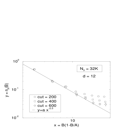
Figure 3: Volume distribution of minbu in terms of the spherical boundary surfaces in 3D DT mfds at distance 11. Total volume of 3D DT mfds is 32K. There are several lower limits of the volume of the spherical boundary surfaces: 200, 400 and 600.

The following question now arises: how to measure $\gamma_{st}$ of these boundary surfaces with different sizes. Suppose that a spherical boundary surface with area $A$ is obtained; we can then use the standard minbu algorithm[13] in order to measure $\gamma_{st}$. The distribution function for the minbu with size $B$ can be written as

$$n_{A}(B)=\frac{3(A-B+1)(B+1)Z[A-B+1]Z[B+1]}{Z[A]}.$$ (5)

When we substitute the asymptotic form of the partition function, $Z[A]\approx A^{\gamma_{st}-3}e^{\mu A}$, for eq.(5) we obtain the normalized distribution function,

$$n_{A}(B)=c\left\{(B+1)(1-\frac{B-1}{A})\right\}^{\gamma_{st}-2},$$ (6)

where c denotes a normalization factor which depends on the area ($A$). The spherical mother boundaries are selected as grand-canonical ensembles. In the case that the topology of the boundary surface is not a sphere, but a handle-body, such as a torus, the standard minbu algorithm does not work well. It is for this reason that we concentrate on the spherical boundary surface.

There are other things to note in terms of the grand-canonical ensembles in question. Using the grand-canonical ensembles for the measurement $\gamma_{st}$ of boundary surfaces, we suffer from finite-size effects. Therefore, we should introduce a lower limit of the sizes of the boundary surfaces. Then, the grand-canonical ensemble does not contain surfaces whose sizes are less than the lower limit. We choose an appropriate geodesic distance corresponding to the total volume ($N_{3}$).

Fig.2 shows the distribution of the minbu of the spherical mother boundary surfaces at d$=10$ with a total volume ($N_{3}$) of $16K$. Fig.3 shows the distribution of the minbu of the spherical mother boundary surfaces at d$=11$ with $N_{3}=32K$. Whether those introduced lower limits are sufficient or not is open to question, and the average size of the grand-canonical ensembles is about $700$ for lower limit of $600$ in Fig.3. We examed separately the string susceptibility exponent in two-dimensional pure gravity with a total area of $700$, and actually obtained $\gamma_{st}=-0.49(5)$ with the number of ensembles being $10^{5}$, even in such a small-size simulation. Fig.3 reveals that the scaling property of the minbu area distributions becomes more clear the bigger is the average size of the boundary. Thus, these distributions remain after the thermal limit $N_{3}\to\infty$. It should be concluded, due to these scaling relations, that the string susceptibility exponent of the spherical mother boundary surfaces in three dimensions is completely consistent with the string susceptibility exponent of the random surface in two dimensions. Our numerical results given here agree with the discussions in refs. [14, 15].

On the other hand, when we apply the method in the previous section to higher dimensions, we are confronted by a difficulty. We cannot use Euler’s character in order to distinguish the topologies of three-dimensional DT mfds. That is to say, to chose a spherical three-dimensional boundary mfd in four-dimensional mfd is not easy at all. Thus, it is difficult to determine $\gamma_{st}$ of the boundary mfds in four dimensions by means of the minbu technique because of the reason mentioned above. It is too involved a subject to be treated here in detail.

Thus in the following section we consider the scaling structures of the minbu distributions in three- and four-dimensional simplicial quantum gravity.

4 Fractal structures of three- and four-dimensional DT mfds

In the introduction we report on the possibility that this model in three- and four-dimensional simplicial quantum gravity makes sense near to the critical point belonging to the strong-coupling phase. Therefore, we investigated the scaling structures of the minbu distributions near to the critical point belonging to the strong coupling phase numerically. Fig.4 shows the distribution of the minbu of three-dimensional DT mfds with a total volume ($N_{3}$) of $16K$. We tune $\kappa_{0}=4.09$ and $\kappa_{3}=2.20$. The three branches shown in Fig.4 reflect the symmetric factor of three-dimensional DT mfds. The influence of such a symmetric factor has not been observed in two-dimensional DT surfaces. Fig.5 shows the distribution of minbu of four-dimensional DT mfds with a total volume ($N_{4}$) of $64K$. We tune $\kappa_{2}=1.275$ and $\kappa_{4}=1.353$. We also observe two branches which reflect the symmetric factor of four-dimensional DT mfds. In three and four dimensions we have a similar scaling behaviour of the minbu volume. From these scaling date which are shown in Figs.4, 5, we can extract the string susceptibility exponents: $\gamma_{st}=-0.05(6)$ with $N_{3}=16K$ and $\gamma_{st}=0.26(5)$ with $N_{4}=64K$[16].

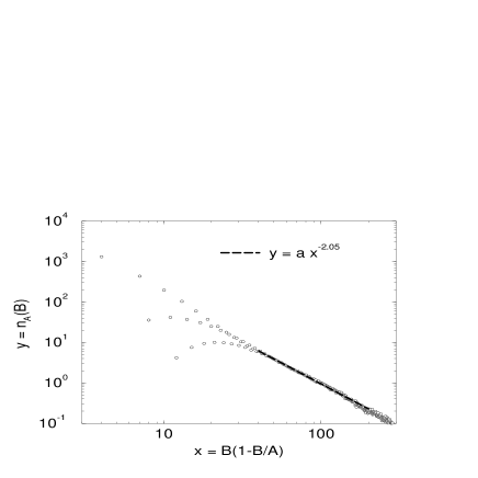
Figure 4: Minbu volume distribution $n_{A}(B)$ of the three-dimensional DT mfds with $N_{3}=16K$ with log-log scales. Coupling constants $\kappa_{0}=4.09$ and $\kappa_{3}=2.20$ for $N_{3}=16K$. Dotted line is drown using the least squares with the data points of $800$ configurations with a range of (x=)$40\sim 200$.

Figure 5: Minbu volume distribution $n_{A}(B)$ of the four-dimensional DT mfds with $N_{4}=64K$ with log-log scales. Coupling constants $\kappa_{2}=1.275$ and $\kappa_{4}=1.353$ for $N_{4}=64K$. Dotted line is drown using the least squares with the data points of $500$ configurations with a range of (x=)$40\sim 1000$.

4.1 Continuum limit in four-dimensional pure simplicial quantum gravity

It is generally agreed that the phase transition of simplicial quantum gravity in both three and four dimensions is first order[8, 9]. Why is the scaling behaviour observed near to the critical point? Let us devote a little more space to discussing this question. In ref.[17] a quantum theory of four-dimensional gravity which is the analog of the Liouville theory of two-dimensional quantum gravity has been argued by considering the effective action for the conformal factor of the metric induced by the four-dimensional trace anomaly. The authors in the reference have also argued for a model including the volume (cosmological constant) and Einstein terms. The string susceptibility exponent ($\gamma_{st}$) obtained by ref.[17] in four dimensions has a similar behaviour to the $\gamma_{st}$ obtained by the Liouville theory in two dimensions:

$$\gamma_{st}(Q^{2})=-\frac{Q^{2}}{4}(1-\frac{8}{Q^{2}}+\sqrt{1-\frac{8}{Q^{2}}})\;\;\;(4\;\mbox{Dim})$$ (7)

and

$$\gamma_{st}(c)=-\frac{1}{12}(1-c+\sqrt{(1-c)(25-c)})\;\;\;(2\;\mbox{Dim}).$$ (8)

Here, $Q^{2}$ which plays the role analogous to matter central charge in two dimensions is the coefficient of the Gauss-Bonnet term in the trace anomaly[17]. If $Q^{2}>8$ (i.e., $\gamma_{st}(Q^{2})<0$, the cosmological and the Einstein terms become irrelevant in the infinite volume limit, and the spike configurations are suppressed[17]. Smooth configuration (i.e. smooth phase) is expected to appear. $Q^{2}=8$ ($\gamma_{st}=0$) behaves in many respects like the $c=1$ case in two-dimensional quantum gravity.

Our numerical results mentioned in the previous subsection, as shown in Fig.6, suggest that there are no signals for the smooth phase in which we can take the continuum limit.

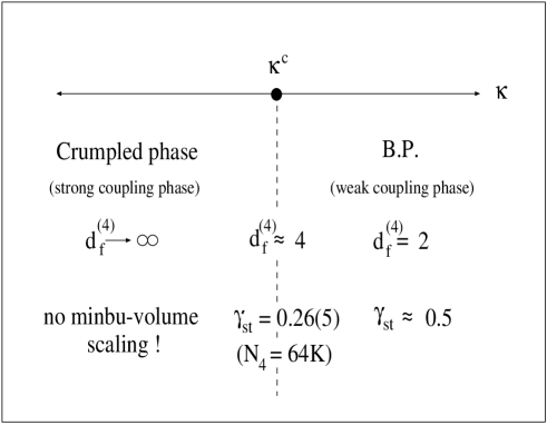
Figure 6: Phase diagram expected from numerical simulations for pure 4D simplicial gravity. $d^{(4)}_{f}$ indicates the fractal dimension obtained in 4D.

It seems reasonable to suppose that the scaling relations which we obtained near to the critical point are pseudo-scaling relations.

5 Summary and Discussion

We investigated the statistical properties of boundary surfaces of three-dimensional DT mfds with $S^{3}$ topology near to the critical point. We have found positive evidence that the spherical mother boundary surfaces in three dimensions are equivalent to two-dimensional spherical random surfaces described by the matrix model. We thus have a conjecture: the mother boundary surfaces in three dimensions with any handles are statistically equivalent to two-dimensional random surfaces described by the matrix model. Therefore, if these boundary surfaces in three dimensions can be recognized as random surfaces, three-dimensional DT mfds can be reconstructed by the direct products of $\Sigma$ (two-dimensional DT surfaces) and $d$ (geodesic distance). Unfortunately, we cannot use the Euler’s character in order to distinguish the topologies of three-dimensional DT mfds. Thus, it is difficult to determine $\gamma_{st}$ of the boundary mfds in four dimension by means of the minbu technique. There is room for further investigation.

Furthermore, we investigated the volume distributions of the minbu of three- and four-dimensional DT mfd near to the critical point. Our numerical results of the minbu volume distribution in three and four dimensions show a tendency which is also similar to two-dimensional case. If we assume that the partition function in three and four dimensions can be written in the same asymptotic form as the two-dimensional case, we obtain the string susceptibility exponents: $\gamma_{st}=-0.05(6)$ with $N_{3}=16K$ and $\gamma_{st}=0.26(5)$ with $N_{4}=64K$ near to the critical point.

Acknowledgements

We are grateful to H.Kawai, H.Hagura, N.Ishibashi, T.Izubuchi and Y.Watabiki for useful discussions and comments. One of the authors (N.T.) is supported by Research Fellowships of the Japan Society for the Promotion of Science for Young Scientists.

References

- [1] E.Brézin and V.Kazakov, Phys.Lett. B236 (1990) 144; M.Douglas and S.Shenker, Nucl.Phys. B335 (1990) 635; D.Gross and A.Migdal, Phys.Rev.Lett. 64 (1990) 127.
- [2] V.G.Knizhnik, A.M.Polyakov and A.B.Zamolodchikov, Mod.Phys.Lett A, Vol.3 (1988) 819; J.Distler and H.Kawai, Nucl.Phys. B321 (1989) 509. F.David, Mod.Phys.Lett. A3 (1988) 1651.
- [3] D.Weingarten, Nucl.Phys. B210 (1982) 229; F.David, Nucl.Phys. B257[FS14] (1985) 45; V.A.Kazakov, Phys.Lett. B150 (1985) 282; J.Ambjørn, B.Durhuus and J.Frhlich, Nucl.Phys.B257 [FS14] (1985) 433; Nucl.Phys. B275 [FS17] (1986) 161; M.E.Agishtein and A.A.Migdal, Nucl.Phys. B350 (1991) 690.
- [4] J.Ambjørn,and S.Varsted, Phys.Lett. B266 (1991) 285; J Ambjørn, B.Durhuus and T.Jonsson, Mod.Phys.Lett. A 6 (1991) 1133; M.E.Agishtein and A.A.Migdal, Mod.Phys.Lett. A 6 (1991) 1863; D.V.Boulatov and A.Krzywicki, Mod.Phys.Lett. A 6 (1991) 3005; S.Varsted, Nucl.Phys. B (Proc.Suppl.) 26 (1992) 578; S.Catterall, J.Kogut and R.Renken, Phys.Lett. B342 (1995) 53.
- [5] H.Hagura, N.Tsuda and T.Yukawa, hep-lat/9512016, to be published in Phys.Lett. B.
- [6] H.S.Egawa, T.Hotta, T.Izubuchi, N.Tsuda and T.Yukawa, Prog.Theor.Phys. 97 (1997) 539; Nucl.Phys. B (Proc.Suppl.) 53 (1997) 760; B.V.Bakker and J.Smit, Nucl.Phys. B439 (1995) 239; J.Ambjørn and J.Jurkiewicz, Nucl.Phys. B451 (1995) 643.
- [7] H.Kawai and M.Ninomiya, Nucl.Phys. B336 (1990) 115; N.Kawamoto, V.Kazakov, Y.Saeki and Y.Watabiki, Phys.Rev.Lett. 68 (1992) 2113. N.Tsuda and T.Yukawa, Phys.Lett. B305 (1993) 223; H.Kawai, N.Kawamoto, T.Mogami, and Y.Watabiki, Phys.Lett. B306 (1993) 19; Y.Watabiki, Nucl.Phys. B441 (1995) 119; J.Ambjørn, J.Jurkiewicz and Y.Watabiki, Nucl.Phys. B454 (1995) 313.
- [8] S.Catterall, J.Kogut and R.Renken, Nucl.Phys. B (Proc.Suppl.) 30 (1993) 775; J.Ambjørn, Z.Burda, J.Jurkiewicz and C.F.Kristjansen, Nucl.Phys. B (Proc.Suppl.) 30 (1993) 771; J.Ambjørn,and S.Varsted, Nucl.Phys. B373 (1992) 557; J.Ambjørn, D.V.Boulatov, A.Krzywicki and S.Varsted, Phys.Lett. B276 (1992) 432.
- [9] B.V.de Bakker, Phys.Lett. B389 (1996) 238; S.Bilke, Z.Burda, A.Krzywicki, B.Petersson, Nucl.Phys. B (Proc.Suppl.) 53 (1997) 743; P.Bialas, Z.Burda, A.Krzywicki, B.Petersson, Nucl.Phys. B472 (1996) 293
- [10] N.Ishibashi and H.Kawai, Phys.Lett. B314 (1993) 190.
- [11] G.K.Savvidy and K.G.Savvidy, Mod.Phys.Lett. A11 (1997) 1379.
- [12] H.S.Egawa and N.Tsuda, Random Surfaces in Three-Dimensional Simplicial Gravity hep-lat/9705020.
- [13] S.Jain and S.D.Mathur, Phys.Lett. B286 (1992) 236.
- [14] H.Verlinde, Nucl.Phys. B337 (1990) 652.
- [15] N.Ishibashi, UCSBTH-90-72.
- [16] H.S.Egawa, N.Tsuda and T.Yukawa, hep-lat/9709099, to be appeared in Nucl.Phys. B (Proc.Suppl.) 1998.
- [17] I.Antoniadis, P.O.Mazur and E.Mottola, Phys.Lett. B323 (1994) 284.