BUTP-97/36
                                                             UNIGRAZ-UTP-02-02-98

Properties of the Fixed Point Lattice Dirac Operator in the Schwinger Model.

Federico Farchioni
Institute for Theoretical Physics

University of Graz

Universitätsplatz 5, A-8010 Graz, Austria

and

Victor Laliena
Institute for Theoretical Physics

University of Bern

Sidlerstrasse 5, CH-3012 Bern, Switzerland

March 2024

Abstract

We present a numerical study of the properties of the Fixed Point lattice Dirac operator in the Schwinger model. We verify the theoretical bounds on the spectrum, the existence of exact zero modes with definite chirality, and the Index Theorem. We show by explicit computation that it is possible to find an accurate approximation to the Fixed Point Dirac operator containing only very local couplings.

1 Introduction

Lattice QCD is a tool to perform (in principle exact) non-perturbative computations of physical quantities in problems where the strong interaction effects are important, by means of numerical simulations. Yet, available computer resources do not allow simulations on lattices extended over a large enough physical size (to keep the finite size effects under control) and with small enough lattice spacing (to make the non-physical cut off dependence negligible).

In the pure gauge sector, together with the contamination of the physical results by lattice artifacts, we face up to an unpleasant situation: the difficulties in studying the topological effects, a genuinely non-perturbative problem. At the classical level, it is possible to define a lattice topological charge operator which, as in the continuum, assumes integer values on all lattice configurations, the Lüscher’s [1] “geometrical” definition. Unfortunately, at the quantum level this operator displays a singular continuum limit, since it assigns non-zero topological charge to lattice configurations extended over a size which scales with the lattice spacing (these configurations are called in the literature “dislocations”). An alternative approach [2] consists in defining the lattice topological charge operator in terms of a local density, obtained from the naive discretization of the continuum operator. At the classical level, the resulting lattice operator, though not integer-valued, has the right continuum limit. At the quantum level, its matrix elements are connected to those of the continuum by non trivial renormalizations [3]. This approach, relying only on first principles of Quantum Field Theory, is theoretically sound, but it has the inconvenience of the evaluation of the renormalizations, a theoretical uncertainty being introduced as a consequence in the lattice determinations.

Among the cut off effects, those in the fermion sector are specially bothersome. The Nielsen-Ninomiya theorem [4] states the impossibility of finding a local lattice action which is chiral invariant and describes only one species fermion in the continuum limit. A related problem is the impossibility of reproducing the right chiral anomaly in the continuum limit with chirally symmetric lattice actions. Since locality is of utmost importance for practical purposes, any lattice action for QCD must necessarily violate chiral symmetry. This violation is so strong for the simplest discretizations of the fermion action (“Wilson action”, “clover action”) that all the chiral properties of the continuum Dirac operator are lost on the lattice, although they should be recovered in the continuum limit. An example of these properties is, at the classical level, the existence of zero modes with definite helicity, and their relation to the topological charge of the background gauge configuration through the Atiyah-Singer formula (Index Theorem) [5]:

$$Q\;=\;n_{\textstyle\scriptscriptstyle L}\>-\>n_{\textstyle\scriptscriptstyle R}\;\;,$$ (1)

where $Q$ is the topological charge and $n_{\textstyle\scriptscriptstyle L}$ and $n_{\textstyle\scriptscriptstyle R}$ are respectively the number of the left- and right-handed zero modes of the Dirac operator.

At the quantum level, other important diseases are induced by the violation of chiral the symmetry; an example is the necessity of a fine tuning of the parameters to recover the (spontaneously broken) chiral symmetry in the continuum limit (namely to get massless pions, chiral Ward identities, etc.).

The freedom of choosing the lattice action among all possibilities in the universality class of the proper renormalized theory can be exploited in order to reduce the cut off effects at the price of rising the number of couplings involved in the action and their extension in space-time. The reward consists in more accurate physical results from simulations on coarse lattices. The drawback is of course the slowing down of the simulation procedure, due to the increased complexity of the action. Whether all this can be of practical or only academic relevance depends on the effective improvement of the accuracy of the results for a fixed cost in computational time.

It follows as a consequence of the Wilson Renormalization Group (RG) ideas that there exist actions which give exact physical answers no matter how coarse the lattice is, the perfect actions [6]. They are located on the renormalized trajectory of any RG transformation. The first step toward perfect actions is represented by the so called fixed point (FP) actions, which are perfect at the classical level: this means, for asymptotically free theories, in the limit $g\rightarrow 0$, where $g$ is the (asymptotically free) coupling constant. It was shown by Hasenfratz and Niedermayer [7] that the determination of the FP action of an asymptotically free theory is a feasible objective, since it requires only the solution of a classical minimization problem. The FP action is by construction perfect at the classical level, and as a consequence cut off effects are absent in the tree-level term of the perturbative expansion of the spectral quantities of the theory; for some specific observables, one-loop cut off effects are absent [8, 9], or strongly suppressed with respect to a standard discretization [10].

In the context of the SU(3) Yang-Mills theory, the properties of the FP action are by now well known from a theoretical point of view [11], and they have been extensively tested in Monte Carlo simulations [12, 13, 14], with the result of very small cut off effects for spectral quantities even at moderate correlation lengths. Also, the ideas of the RG allow to build a well-defined topological charge operator on the lattice, the FP topological charge operator, which assumes integer values on all gauge configurations and is not affected by topological defects [15, 16].

The next step, the inclusion of quarks, is yet in a preliminary phase [17, 18]. It is theoretically clear [19, 20] that many of the diseases of the simplest fermion actions produced by the violation of the chiral symmetry are cured by working with a FP action, whose (obligatory) chiral asymmetry is so mild that it has no effect in the physical results: the classical statements like the existence of zero modes of topological origin and the Index Theorem hold [20]; at the quantum level, chiral symmetry is recovered at zero bare quark mass, without any tuning of an additional parameter, the currents get no renormalization, and there is no mixing between composite fermion operators corresponding to different chiral representations [21]. This properties are deduced using the Ginsparg-Wilson (GW) relation [22], which expresses the mildest breaking of the chiral symmetry for a “legal” fermion action; this relation is satisfied by any FP Dirac operator. Very recently, Lüscher has pointed out that fermion actions verifying the GW relation have an exact continuous symmetry, which can be interpreted as a lattice implementation of the chiral symmetry without any contradiction with the Nielsen-Ninomiya theorem [23].

It is worth to observe in this context that a solution of GW equation was obtained independently from the RG techniques. This solution is a product of the overlap formalism and shares with the FP Dirac operator its gentle chiral properties [24].

In this paper we want to verify the classical properties of the FP action in the fermion sector in a model simpler than QCD: the Schwinger model. The work is analytical for the pure gauge sector and numerical for the fermion sector. We investigate in particular how the approximation of the FP action with a finite-range fermion matrix affects its (classically perfect) properties. The paper is organized as follows. In Sec. 2 we recall the recursion relation obeyed by the FP Dirac operator, enlightening some properties of its classical solutions and bounds on the spectrum; in particular, we formulate the lattice version of the Index Theorem. In Sec. 3 we describe some topological properties of the continuum Schwinger model relevant for the subsequent work and define the RG transformation which generates the FP action under study, discussing the analytical results of the pure-gauge sector. Sec. 4 is devoted to the discussion of the numerical results concerning the spectrum of the FP Dirac operator. The paper ends with a summary of the conclusions in Sec. 5.

2 The Fixed Point lattice Dirac operator

2.1 Recursion relations

Let us recall schematically how the FP action for asymptotically free gauge theories can be computed; for further details, we refer the reader to the literature [11, 6]. Consider a gauge theory, whose lattice action can be written as

$$S[\,U,\psi,\bar{\psi}\,]\;=\;\beta\,S_{\rm\textstyle\scriptscriptstyle G}(U)\>+\>\sum_{n,m}\,\bar{\psi}_{n}\,\Delta_{nm}(U)\,\psi_{m}\,,$$ (2)

where $S_{\rm\textstyle\scriptscriptstyle G}(U)$ is a lattice action for the pure gauge part, for example the Wilson single plaquette action, and $\Delta(U)$ is a proper discretization of the continuum Dirac operator. On the lattice, the latter operator has the form of a matrix with space-time, Dirac and color indices, which in the above formula have been indicated in a collective notation. Since we do not want replica fermions in the spectrum, $\Delta(U)$ cannot be chiral symmetric, i.e. it must mix-up left- and right-handed spinor components.

We define a physically equivalent action on a lattice with doubled lattice spacing through a RG transformation:

$$\exp\,\left[\,-\,\beta^{\prime}\,S_{\rm\textstyle\scriptscriptstyle G}^{\prime}(U^{\prime})\>-\>S_{\rm\textstyle\scriptscriptstyle F}^{\prime}(\bar{\psi}^{\prime},\psi^{\prime},U^{\prime})\,\right]\;=$$

$$\hskip 28.45274pt\int\,\left[dU\,d\bar{\psi}\,d\psi\right]\,\exp\,\left[-\,\beta\,S_{\rm\textstyle\scriptscriptstyle G}(U)\>-\>\bar{\psi}\,\Delta(U)\,\psi\>-\>p\,{\cal K}_{\rm\textstyle\scriptscriptstyle G}(U^{\prime},U)\right.$$

$$\hskip 28.45274pt\left.-\>\kappa_{\rm\textstyle\scriptscriptstyle F}\,{\cal K}_{\rm\textstyle\scriptscriptstyle F}(\bar{\psi}^{\prime},\psi^{\prime},\bar{\psi},\psi,U)\,\right]\,,$$ (3)

where the primed fields are the degrees of freedom on the coarser lattice, defined through the gauge invariant kernels  ${\cal K}_{\rm\textstyle\scriptscriptstyle G}$  and  ${\cal K}_{\rm\textstyle\scriptscriptstyle F}$. The parameters $p$ and $\kappa_{\rm\textstyle\scriptscriptstyle F}$ can be chosen arbitrarily; in particular, we can take $p=\beta\,\kappa_{\rm\textstyle\scriptscriptstyle G}$, where $\kappa_{\rm\textstyle\scriptscriptstyle G}$ is a fixed parameter. Note that in general the fermion action is not quadratic in the fermion fields after a RG transformation.

In the class of theories under interest (including asymptotically free non-abelian gauge theories and the Schwinger model), the critical surface (where the continuum is attained) is at $\beta=\infty$. The iteration of the RG transformation starting on this surface converges to a FP. When $\beta\rightarrow\infty$ the integral on the gauge degrees of freedom in the r.h.s. of Eq. (3) is saturated by the saddle point configuration; the solution of the recursion is then:

$$S_{\rm\textstyle\scriptscriptstyle G}^{\prime}(U^{\prime})\;=\;\min_{\{U\}}\,\left[S_{\rm\textstyle\scriptscriptstyle G}(U)\>+\>\kappa_{\rm\textstyle\scriptscriptstyle G}\,{\cal K}_{\rm\textstyle\scriptscriptstyle G}(U^{\prime},U)\,\right]\,,$$ (4)

$$S_{\rm\textstyle\scriptscriptstyle F}^{\prime}(\bar{\psi}^{\prime},\psi^{\prime},U^{\prime})\;=\;-\ln\,\int\,\left[d\bar{\psi}\,d\psi\right]\,\exp\,\left[\,-\>\bar{\psi}\,\Delta(U^{\rm\textstyle\scriptscriptstyle min})\,\psi\right.$$

$$\left.\;\;\;\;\;\;\;\;\;\;\;\;\;\;\;\;\;\;\;\;\;\;\;\;\;\;\;\;\;\;\;\;\;\;\;\;-\>\kappa_{\rm\textstyle\scriptscriptstyle F}\,{\cal K}_{\rm\textstyle\scriptscriptstyle F}(\bar{\psi}^{\prime},\psi^{\prime},\bar{\psi},\psi,U(U^{\rm\textstyle\scriptscriptstyle min}))\,\right]\,,$$ (5)

where $U^{\rm\textstyle\scriptscriptstyle min}$ is the fine gauge field configuration which minimizes the r.h.s. of Eq. (4). It depends on the coarse configuration $U^{\prime}$. We have also $\beta^{\prime}=\beta=\infty$. In this limit the problem is equivalent to a classical minimization problem plus a Grassmann integration.

If the fermion kernel is quadratic in the fermion fields, the fermion action at $\beta=\infty$ remains quadratic after a RG transformation, as is evident from Eq. (5). We write in general

$${\cal K}_{\rm\textstyle\scriptscriptstyle F}\;=\;\sum_{x_{\textstyle\scriptscriptstyle b}}\,\left(\,\bar{\psi}^{\prime}_{x_{\textstyle\scriptscriptstyle b}}\>-\>\sum_{x}\,\bar{\psi}_{x}\,\omega_{xx_{\textstyle\scriptscriptstyle b}}^{\dagger}\,\right)\,\left(\,\psi^{\prime}_{x_{\textstyle\scriptscriptstyle b}}\>-\>\sum_{y}\,\omega_{x_{\textstyle\scriptscriptstyle b}y}\,\psi_{y}\,\right)\;\;,$$ (6)

where $x_{\textstyle\scriptscriptstyle b}$ and $x,y$ label the sites in the coarse and the fine lattices respectively; $\omega$ is a matrix in space-time and color indices, depending on the gauge field $U$ in such a way that gauge invariance is preserved, and normalized according to: $\sum_{x}\omega_{x_{\textstyle\scriptscriptstyle b}x}=2^{\frac{d-1}{2}}$. The adjoint operation denoted with the symbol $\dagger$ acts on all indices, including space-time.

The FP action is defined as

$$S^{\rm\scriptscriptstyle FP}\;=\;\beta\,S^{\rm\scriptscriptstyle FP}_{\rm\textstyle\scriptscriptstyle G}(U)\>+\>\bar{\psi}\,\Delta^{\rm\textstyle\scriptscriptstyle FP}(U)\,\psi\,,$$ (7)

where $S^{\rm\scriptscriptstyle FP}_{\rm\textstyle\scriptscriptstyle G}$ and $\Delta^{\rm\scriptscriptstyle FP}$ are the self-reproducing solutions of Eq. (4) and Eq. (5) respectively. The recursion relation for the FP action of the pure gauge sector and for the FP Dirac operator read respectively:

$$S_{\rm\textstyle\scriptscriptstyle G}^{\rm\scriptscriptstyle FP}(U)\;=\;S_{\rm\textstyle\scriptscriptstyle G}^{\rm\scriptscriptstyle FP}(U^{\rm\textstyle\scriptscriptstyle min}(U))\>+\>\kappa_{\rm\textstyle\scriptscriptstyle G}\,{\cal K}_{\rm\textstyle\scriptscriptstyle G}(U,U^{\rm\textstyle\scriptscriptstyle min}(U))\;\;,$$ (8)

$$\Delta^{\rm\scriptscriptstyle FP}_{x_{\textstyle\scriptscriptstyle b}y_{\textstyle\scriptscriptstyle b}}(U)\;=\;\kappa_{\rm\textstyle\scriptscriptstyle F}\,\delta_{x_{\textstyle\scriptscriptstyle b}y_{\textstyle\scriptscriptstyle b}}\>-\>\kappa_{\rm\textstyle\scriptscriptstyle F}^{2}\,\sum_{xy}\,\omega_{x_{\textstyle\scriptscriptstyle b}x}\,\left(\frac{1}{\Delta^{\rm\scriptscriptstyle FP}\,+\,\kappa_{\rm\textstyle\scriptscriptstyle F}\,\omega^{\dagger}\,\omega}\right)_{xy}\,\omega^{\dagger}_{yy_{\textstyle\scriptscriptstyle b}}\,,$$ (9)

where $U^{\rm\textstyle\scriptscriptstyle min}(U)$ indicates the lattice gauge configuration defined on the fine lattice realizing the minimum in the r.h.s of Eq. (8) for a fixed coarse lattice configuration $U$. Notice that, although not explicitly displayed, all the matrices in the r.h.s. of Eq. (9) depend on the coarse gauge configuration $U$ through $U^{\rm\textstyle\scriptscriptstyle min}(U)$.

The recursion relation for the inverse Dirac operator $D\equiv\Delta^{-1}$ - the fermion propagator in the background of the gauge configuration $U$ - is linear and therefore simpler and often more convenient:

$$D^{\rm\textstyle\scriptscriptstyle FP}_{x_{\textstyle\scriptscriptstyle b}y_{\textstyle\scriptscriptstyle b}}(U)\;=\;\sum_{xy}\,\omega_{x_{\textstyle\scriptscriptstyle b}x}(U^{\rm\textstyle\scriptscriptstyle min})\,D^{\rm\textstyle\scriptscriptstyle FP}_{xy}(U^{\rm\textstyle\scriptscriptstyle min})\,\omega^{\dagger}_{yy_{\textstyle\scriptscriptstyle b}}(U^{\rm\textstyle\scriptscriptstyle min})\>+\>\frac{1}{\kappa_{\rm\textstyle\scriptscriptstyle F}}\,\delta_{x_{\textstyle\scriptscriptstyle b}y_{\textstyle\scriptscriptstyle b}}\;\;.$$ (10)

2.2 Fixed point operators

Suppose $O(U)$ to be some lattice discretization of a continuum operator depending only on the gauge fields. The RG transformation for such operator reads [25]:

$$\lambda\,O^{\prime}(U^{\prime})\,\exp\,\left[\,-\,\beta^{\prime}\,S_{\rm\textstyle\scriptscriptstyle G}^{\prime}(U^{\prime})\>-\>S_{\rm\textstyle\scriptscriptstyle F}^{\prime}(\bar{\psi}^{\prime},\psi^{\prime},U^{\prime})\,\right]\;=$$

$$\hskip 28.45274pt\int\,\left[dU\,d\bar{\psi}\,d\psi\right]\,O(U)\,\exp\,\left[-\,\beta\,S_{\rm\textstyle\scriptscriptstyle G}(U)\>-\>\bar{\psi}\,\Delta(U)\,\psi\>-\>p\,{\cal K}_{\rm\textstyle\scriptscriptstyle G}(U^{\prime},U)\right.$$

$$\hskip 28.45274pt\left.-\>\kappa_{\rm\textstyle\scriptscriptstyle F}\,{\cal K}_{\rm\textstyle\scriptscriptstyle F}(\bar{\psi}^{\prime},\psi^{\prime},\bar{\psi},\psi,U)\,\right]\;\;,$$ (11)

where the eigenvalue $\lambda$ is determined by dimensional considerations. This relation preserves (apart from a trivial multiplicative factor) the matrix elements of the operator $O(U)$ if, of course, also the action is changed accordingly.

In the $\beta\rightarrow\infty$ limit, if the action is at the FP, the above equation reduces to:

$$\lambda\,O^{\prime}(U^{\prime})\;=\;O(U^{\rm\textstyle\scriptscriptstyle min}(U^{\prime}))\;\;.$$ (12)

Eq. (12) has a FP in the operator $O^{\rm\scriptscriptstyle FP}(U)$ formally defined by the following limit:

$$O^{\rm\scriptscriptstyle FP}(U)=\lim_{n\rightarrow\infty}(1/\lambda)^{n}O(U^{\textstyle\scriptscriptstyle(n)}(U))\;\;,$$ (13)

where $U^{\textstyle\scriptscriptstyle(n)}(U)$ is obtained by applying $n$ times - in a recursive way - Eq. (8) starting from the coarse configuration $U$:

$$U^{\textstyle\scriptscriptstyle(i)}\;=\;U^{\rm\textstyle\scriptscriptstyle min}(U^{\textstyle\scriptscriptstyle(i-1)})\;\;\;\;\;{\rm and}\;\;\;\;\;U^{\textstyle\scriptscriptstyle(0)}\;\equiv\;U\,.$$ (14)

As is evident from the definition (13), the FP operator $O^{\rm\scriptscriptstyle FP}$ is the solution of the FP equation:

$$\lambda\,O^{\rm\scriptscriptstyle FP}(U)\;=\;O^{\rm\scriptscriptstyle FP}(U^{\rm\textstyle\scriptscriptstyle min}(U))\;\;.$$ (15)

$O^{\rm\scriptscriptstyle FP}(U)$ represents the classical perfect lattice operator, in the sense that its classical properties are the same of the corresponding continuum operator.

A case of particular interest is that of the topological charge operator. Indeed, the FP charge operator $Q^{\rm\scriptscriptstyle FP}(U)$ allows a theoretically sound definition of the topology on the lattice, since it assumes integer values and it is not affected by short-range fluctuations (“dislocations”) [15, 16].

2.3 Classical solutions and the Index Theorem

In analogy with the pure-gauge sector, where there exist exact classical solutions of the lattice equations of motion having the main properties of the continuum solutions (e.g. scale invariance) [11], it is also possible to prove [19] the existence of exact solutions of the lattice FP Dirac equation, given by the zero modes of the FP Dirac operator. The arguments given here follow [19]; see also [20] for an alternative approach.

Suppose $f^{\textstyle\scriptscriptstyle(c)}_{x_{\textstyle\scriptscriptstyle b}}$ to be a solution of the FP Dirac equation in the background of some coarse configuration $U^{\textstyle\scriptscriptstyle(c)}$ (Dirac and color indices are understood):

$$\sum_{y_{\textstyle\scriptscriptstyle b}}\,\Delta^{\rm\scriptscriptstyle FP}_{x_{\textstyle\scriptscriptstyle b}y_{\textstyle\scriptscriptstyle b}}(U^{\textstyle\scriptscriptstyle(c)})\,f^{\textstyle\scriptscriptstyle(c)}_{y_{\textstyle\scriptscriptstyle b}}\;=\;0\;\;.$$ (16)

Using (9) it is easy to verify that

$$f^{\textstyle\scriptscriptstyle(f)}_{x}\;=\;\sum_{yy_{B}}\,\left(\frac{1}{\Delta^{\rm\scriptscriptstyle FP}(U^{\rm\textstyle\scriptscriptstyle min})\,+\,\kappa_{\rm\textstyle\scriptscriptstyle F}\,\omega^{\dagger}(U^{\rm\textstyle\scriptscriptstyle min})\omega(U^{\rm\textstyle\scriptscriptstyle min})}\right)_{xy}\,\omega^{\dagger}_{yy_{B}}(U^{\rm\textstyle\scriptscriptstyle min})\,f^{\textstyle\scriptscriptstyle(c)}_{y_{B}}$$ (17)

is also a solution of the Dirac equation in the fine lattice with the background configuration $U^{\rm\textstyle\scriptscriptstyle min}(U^{\textstyle\scriptscriptstyle(c)})$:

$$\sum_{y}\,\Delta^{\rm\scriptscriptstyle FP}_{xy}(U^{\rm\textstyle\scriptscriptstyle min}(U^{\textstyle\scriptscriptstyle(c)}))\,f^{\textstyle\scriptscriptstyle(f)}_{y}\;=\;0$$ (18)

Conversely, let $f^{\textstyle\scriptscriptstyle(f)}_{x}$ be a solution of the Dirac equation in the fine lattice, with the background configuration $U^{\rm\textstyle\scriptscriptstyle min}(U^{\textstyle\scriptscriptstyle(c)})$. Then

$$f^{\textstyle\scriptscriptstyle(c)}_{x_{\textstyle\scriptscriptstyle b}}\;=\;\sum_{x}\,\omega_{x_{\textstyle\scriptscriptstyle b}x}(U^{\rm\textstyle\scriptscriptstyle min})\,f^{\textstyle\scriptscriptstyle(f)}_{x}$$ (19)

is a solution of the Dirac equation in the coarse lattice with the background configuration $U^{\textstyle\scriptscriptstyle(c)}$.

Eqs. (17) and (19) establish a one-to-one correspondence between the zero modes of the FP Dirac operator in the background of the coarse gauge configuration $U^{\textstyle\scriptscriptstyle(c)}$ with those of the same operator, but considered now in the background of the fine gauge configuration $U^{\rm\textstyle\scriptscriptstyle min}(U^{\textstyle\scriptscriptstyle(c)})$. From Eq. (19) we see that two related zero modes must have the same chirality, since $\omega$ does not depend on Dirac indices. By iteration, one can relate in the same way the zero modes of $\Delta^{\rm\scriptscriptstyle FP}_{xy}(U^{\textstyle\scriptscriptstyle(c)})$ to those of $\Delta^{\rm\scriptscriptstyle FP}_{xy}(U^{\textstyle\scriptscriptstyle(n)}(U^{\textstyle\scriptscriptstyle(c)}))$, where $U^{\textstyle\scriptscriptstyle(n)}(U^{\textstyle\scriptscriptstyle(c)})$ is defined as in Eq. (14). In the limit of infinite iterations $n\rightarrow\infty$, $U^{\textstyle\scriptscriptstyle(n)}(U^{\textstyle\scriptscriptstyle(c)})$ converges to a continuous configuration. The topological charge of such configuration is given by

$$Q=\lim_{n\rightarrow\infty}Q^{L}(U^{\textstyle\scriptscriptstyle(n)}(U^{\textstyle\scriptscriptstyle(c)}))\;\;,$$ (20)

where $Q^{L}$ indicates any proper lattice discretization of the topological charge operator. The r.h.s. of the above equation is just the definition of the FP topological charge of the coarse lattice configuration $U^{\textstyle\scriptscriptstyle(c)}$, $Q^{\rm\scriptscriptstyle FP}(U^{\textstyle\scriptscriptstyle(c)})$ (see Eq. (13); in the case of the topological charge, a dimensionless operator, $\lambda=1$). For the limiting continuous configuration the Index Theorem holds, since $\Delta^{\rm\scriptscriptstyle FP}_{xy}(U^{\textstyle\scriptscriptstyle(n)})$ converges to the continuum operator when $n\rightarrow\infty$. Using the above established one-to-one correspondence between the zero modes, and the fact that this correspondence preserves chirality, we arrive to the conclusion that [19, 20]:

• the FP Dirac operator $\Delta^{\rm\scriptscriptstyle FP}(U)$ possesses exact zero modes of topological origin;

• these zero modes have definite chirality and satisfy the Index Theorem, if the lattice topological charge is the FP topological charge $Q^{\rm\scriptscriptstyle FP}(U)$ of the background lattice gauge configuration $U$.

2.4 The Ginsparg-Wilson relation

Let us show now how, forced by the Nielsen-Ninomiya theorem, the FP Dirac operator violates the chiral symmetry [19, 20]. Consider the n-th iteration of Eq. (10):

$$D^{\rm\textstyle\scriptscriptstyle FP}_{x_{\textstyle\scriptscriptstyle b}y_{\textstyle\scriptscriptstyle b}}(U)\;=\;\sum_{xy}\,\Omega^{\textstyle\scriptscriptstyle(n)}_{x_{\textstyle\scriptscriptstyle b}x}(U)\,D^{\rm\textstyle\scriptscriptstyle FP}_{xy}(U^{\textstyle\scriptscriptstyle(n)})\,\Omega^{{\textstyle\scriptscriptstyle(n)}\,\dagger}_{yy_{\textstyle\scriptscriptstyle b}}(U)\>+\>R^{\textstyle\scriptscriptstyle(n)}_{x_{\textstyle\scriptscriptstyle b}y_{\textstyle\scriptscriptstyle b}}(U)\,,$$ (21)

where

$$R^{\textstyle\scriptscriptstyle(n)}_{x_{\textstyle\scriptscriptstyle b}y_{\textstyle\scriptscriptstyle b}}(U)\;=\;\frac{1}{\kappa_{\rm\textstyle\scriptscriptstyle F}}\left(\delta_{x_{\textstyle\scriptscriptstyle b}y_{\textstyle\scriptscriptstyle b}}\>+\>\sum_{i=1}^{n-1}\,\sum_{x}\,\Omega^{\textstyle\scriptscriptstyle(i)}_{x_{\textstyle\scriptscriptstyle b}x}\,\Omega^{{\textstyle\scriptscriptstyle(i)}\,\dagger}_{xy_{\textstyle\scriptscriptstyle b}}(U)\right)$$ (22)

and

$$\Omega^{\textstyle\scriptscriptstyle(i)}_{x_{\textstyle\scriptscriptstyle b}x}(U)\;=\;\sum_{x_{1}\ldots x_{i-1}}\,\omega_{x_{\textstyle\scriptscriptstyle b}x_{1}}(U^{\textstyle\scriptscriptstyle(1)})\,\omega_{x_{1}x_{2}}(U^{\textstyle\scriptscriptstyle(2)})\ldots\omega_{x_{i-1}x}(U^{\textstyle\scriptscriptstyle(i)})\,,$$ (23)

with $U^{\textstyle\scriptscriptstyle(i)}(U)$ defined as in Eq. (14).

The background configuration $U^{\textstyle\scriptscriptstyle(n)}$ in Eq. (21) becomes arbitrarily smooth when increasing $n$. Therefore, when $n\rightarrow\infty$ the propagator in the r.h.s. of (21) converges to the continuum propagator, which is chiral invariant. Since $\Omega^{\textstyle\scriptscriptstyle(n)}$ commutes with $\gamma_{5}$ (we recall that $\omega$ does not act on Dirac indices), we have [19]

$$\{\,D^{\rm\textstyle\scriptscriptstyle FP}_{x_{\textstyle\scriptscriptstyle b}y_{\textstyle\scriptscriptstyle b}},\,\gamma_{5}\,\}\;=\;2\,\gamma_{5}\,R^{\rm\textstyle\scriptscriptstyle FP}_{x_{\textstyle\scriptscriptstyle b}y_{\textstyle\scriptscriptstyle b}}(U)\,,$$ (24)

where $R^{\rm\textstyle\scriptscriptstyle FP}$ the limit $n\rightarrow\infty$ of $R^{\textstyle\scriptscriptstyle(n)}$. Equivalently, we have

$$\{\,\Delta^{\rm\scriptscriptstyle FP}_{x_{\textstyle\scriptscriptstyle b}y_{\textstyle\scriptscriptstyle b}},\,\gamma_{5}\,\}\;=\;2\,\left(\,\Delta^{\rm\scriptscriptstyle FP}\,\gamma_{5}\,R^{\rm\textstyle\scriptscriptstyle FP}\,\Delta^{\rm\scriptscriptstyle FP}\,\right)_{x_{\textstyle\scriptscriptstyle b}y_{\textstyle\scriptscriptstyle b}}\;\;.$$ (25)

The hermitian matrix $R^{\rm\textstyle\scriptscriptstyle FP}_{x_{\textstyle\scriptscriptstyle b}y_{\textstyle\scriptscriptstyle b}}$ is local and its spectrum is bounded [20]:

$$1\;\leq\;\kappa_{\rm\textstyle\scriptscriptstyle F}\,\frac{(v,R^{\rm\textstyle\scriptscriptstyle FP}v)}{(v,v)}\;\leq\;\frac{1}{1-q}\;\;,\;\;\;\;0\leq q<1\;\;;$$ (26)

the lower bound comes trivially from Eq. (22), while the upper bound (specifically the constant $q$) is RG-transformation-dependent. In the case of the overlapping-symmetric fermion RG transformation [17, 26], and its gauge-invariant extension for the interacting theory [9] here considered (see the following), one has $q=1/2$.

Ginsparg and Wilson proved [22] that any lattice discretization of the Dirac operator which verifies Eqs. of the form (24)-(25) - it is crucial the locality of the matrix $R^{\rm\textstyle\scriptscriptstyle FP}_{x_{\textstyle\scriptscriptstyle b}y_{\textstyle\scriptscriptstyle b}}$ - reproduces the correct axial anomaly in the continuum limit. We refer Eqs. (24)-(25) as the Ginsparg-Wilson relation (GWR). It expresses the explicit violation of chiral symmetry by the lattice regulator. The fact that this violation takes the form of the GWR ensures that many important chiral properties of the continuum Dirac operator hold also for its FP discretization.

For instance, using the GWR the Index Theorem has been proven in Ref. [20] directly on the lattice, without any reference to the Theorem of the continuum, finding also the following relation between the FP topological charge and the FP Dirac operator:

$$Q^{\rm\textstyle\scriptscriptstyle FP}(U)\;=\;-\frac{1}{2}\,{\rm tr}\left(\gamma_{5}\,\{\Delta^{\rm\scriptscriptstyle FP}(U),\,R^{\rm\textstyle\scriptscriptstyle FP}(U)\}\right)\,.$$ (27)

2.5 About the spectrum

The GWR strongly constrains the spectrum of the FP Dirac operator. Consider first the zero modes. Let us denote by $v$ a vector column which contains the spatial, Dirac and color indices.

Property:
$v$ is a zero mode of $\Delta^{\rm\scriptscriptstyle FP}$ if and only if $\gamma_{5}\,v$ is. Therefore, the zero modes can be chosen eigenstates of $\gamma_{5}$.

The proof is trivial using (25):

$$\Delta^{\rm\scriptscriptstyle FP}\,\gamma_{5}\,v\;=\;-\gamma_{5}\,\Delta^{\rm\scriptscriptstyle FP}\,v\>+\>\{\Delta^{\rm\scriptscriptstyle FP},\,\gamma_{5}\}\,v\;=\;0\;\;.$$ (28)

In what follows we shall prove that the FP Dirac operator is bounded, and we shall find the explicit bound on the spectrum. First, we notice that the FP Dirac operator verifies the hermiticity condition

$$\Delta^{{\rm\scriptscriptstyle FP}\,\dagger}\;=\;\gamma_{5}\,\Delta^{\rm\scriptscriptstyle FP}\,\gamma_{5}\,,$$ (29)

since it is preserved by the recursion relation (6). The hermiticity property, which also holds for the Wilson Dirac operator, implies that the eigenvalues of $\Delta^{\rm\scriptscriptstyle FP}$ are either real or comes by pairs of complex conjugate numbers. It also implies that if $v$ is an eigenvector corresponding to a non real eigenvalue $\lambda$ ($\lambda\neq\lambda^{*}$) then

$$(v,\gamma_{5}v)\;=\;0\;\;.$$ (30)

Multiplying on the left by $\gamma_{5}$ both sides of (25) and using (29), we obtain:

$$\Delta^{\rm\scriptscriptstyle FP}\>+\>\Delta^{{\rm\scriptscriptstyle FP}\,\dagger}\;=\;2\,\Delta^{{\rm\scriptscriptstyle FP}\,\dagger}\,R^{\rm\textstyle\scriptscriptstyle FP}\,\Delta^{\rm\scriptscriptstyle FP}\,.$$ (31)

Let $v$ be an eigenvector of $\Delta^{\rm\scriptscriptstyle FP}$ with eigenvalue $\lambda$, normalized to unity: $(v,v)=1$. Multiplying both sides of (31) by $v^{\dagger}$ on the left and by $v$ on the right, we find:

$$\lambda\>+\>\lambda^{*}\;=\;2\,(v,R^{\rm\textstyle\scriptscriptstyle FP}v)\,|\lambda|^{2}\;\;.$$ (32)

The above equation, in conjunction with the bounds (26) for the $R^{\rm\textstyle\scriptscriptstyle FP}$ matrix, allows to state analogous bounds for the spectrum of the FP Dirac operator [20]:

$$\frac{2}{\kappa_{\rm\textstyle\scriptscriptstyle F}}\,|\lambda|^{2}\;\leq\;\lambda\>+\>\lambda^{*}\;\leq\;\frac{2}{(1-q)\,\kappa_{\rm\textstyle\scriptscriptstyle F}}\>|\lambda|^{2}\;\;.$$ (33)

These inequalities mean that the spectrum of the FP Dirac operator lies in the complex plane inside a circle of radius $\kappa_{\rm\textstyle\scriptscriptstyle F}/2$ centered at $(\kappa_{\rm\textstyle\scriptscriptstyle F}/2,0)$, and outside a circle of radius $(1-q)\,\kappa_{\rm\textstyle\scriptscriptstyle F}/2$ centered at $((1-q)\,\kappa_{\rm\textstyle\scriptscriptstyle F}/2,0)$.

3 The case of the Schwinger model

3.1 Topological properties of Schwinger model

The Schwinger model is a good laboratory to test all these ideas, since it is much simpler than four-dimensional non-abelian gauge theories, but still its gauge sector has non-trivial topology. The topological charge of a gauge configuration $A_{\mu}$ is given by:

$$Q\;=\;\frac{e}{2\pi}\,\int d^{2}x\,F_{\textstyle\scriptscriptstyle 12}\;\;,$$ (34)

where: $F_{\textstyle\scriptscriptstyle 12}=\partial_{\textstyle\scriptscriptstyle 1}A_{\textstyle\scriptscriptstyle 2}-\partial_{\textstyle\scriptscriptstyle 2}A_{\textstyle\scriptscriptstyle 1}$ and $e$ is the electric charge. For the theory defined on a torus $T^{2}$ ($\,x_{\mu}\in[0,L_{\mu}],\,\mu=1,2\,$), topologically non-trivial configurations must necessarily have a jump at the boundary. Of course, gauge invariant functionals of the gauge fields must be continuous. The simplest topologically non-trivial gauge configurations are solutions of the classical equations of motion, therefore with constant $F_{\textstyle\scriptscriptstyle 12}$; in this case a possible expression for the gauge fields is [27]:

$$A^{{\rm\scriptscriptstyle inst}}_{\textstyle\scriptscriptstyle 1}(x)\;=\;-\,\Phi\,x_{\textstyle\scriptscriptstyle 2}\,,\;\;\;\;\;\;\;\;\;\;\;\;\;A^{\rm\scriptscriptstyle inst}_{\textstyle\scriptscriptstyle 2}(x)\;=\;0\,,\;\;\;\;\;\;\;\;\;\;\;\;\;\;\;F_{\textstyle\scriptscriptstyle 12}\;=\;\Phi\;.$$ (35)

The fields $A^{\rm\scriptscriptstyle inst}_{\textstyle\scriptscriptstyle 1}(x_{\textstyle\scriptscriptstyle 2}=L_{\textstyle\scriptscriptstyle 2})$ and $A^{\rm\scriptscriptstyle inst}_{1}(x_{\textstyle\scriptscriptstyle 2}=0)$ can be connected by a transition function (ensuring continuity for gauge-invariant quantities) if $\Phi=2\pi Q/(L_{1}L_{2}e)$, with $Q$ some integer number, corresponding to the topological charge of the gauge configuration on the torus according to definition (34).

In perfect analogy to the case of QCD, also in the Schwinger model it is possible to relate the chiral properties of the zero-modes of the massless Dirac operator to the topological properties of the background gauge configuration $A_{\mu}$. This relation is given by the Atiyah-Singer Index theorem, Eq. (1). A peculiarity of two space-time dimensions is that:

$$Q(A)\;>\;0\;\Rightarrow\;n_{\textstyle\scriptscriptstyle R}\;=\;0\;\;,$$

$$Q(A)\;<\;0\;\Rightarrow\;n_{\textstyle\scriptscriptstyle L}\;=\;0\;\;,$$ (36)

the so called “Vanishing Theorem” [28]. So, in the case $Q(A)\neq 0$, the zero modes have all the same chirality, given by the sign of $Q(A)$.

3.2 The pure gauge sector on the lattice

To be able to study the topological properties of the Schwinger model on the lattice, we discretize the theory in the compact formulation, where the lattice gauge fields are described by angular variables $\alpha_{\mu}(x)\in(-\pi,\,\pi]$ and, forced by the necessity of preserving gauge invariance, the fermions are coupled to the gauge fields through $U(1)$ elements of the form:

$$U_{\mu}(x)\;=\;{\rm e}^{i\,\alpha_{\mu}(x)}\;\;.$$ (37)

The lattice action must be a periodic function of $\alpha_{\mu}$. Within this formulation, we can implement periodic boundary conditions also for the topologically non-trivial gauge field configurations. The lattice discretization of the continuum instanton solution on the torus (35) is [29]:

$$\alpha^{\rm\scriptscriptstyle inst}_{\textstyle\scriptscriptstyle 1}(x) = -\Phi^{\textstyle\scriptscriptstyle L}\,x_{\textstyle\scriptscriptstyle 2}\;({\rm mod}\,2\pi)$$

$$\alpha^{\rm\scriptscriptstyle inst}_{\textstyle\scriptscriptstyle 2}(x) = 0\hskip 106.9822pt{\rm if}\;\;x_{\textstyle\scriptscriptstyle 2}=0,1,\ldots,N_{\textstyle\scriptscriptstyle 2}-2$$

$$= \Phi^{\textstyle\scriptscriptstyle L}N_{\textstyle\scriptscriptstyle 2}\,x_{\textstyle\scriptscriptstyle 1}\;({\rm mod}\,2\pi)\hskip 28.45274pt\;\;{\rm if}\;\;x_{\textstyle\scriptscriptstyle 2}=N_{\textstyle\scriptscriptstyle 2}-1\,,$$ (38)

where $\Phi^{\textstyle\scriptscriptstyle L}=2\pi Q/(N_{\textstyle\scriptscriptstyle 1}N_{\textstyle\scriptscriptstyle 2})$ and $[\theta\;({\rm mod}\,2\pi)]\,\in(-\pi,\,\pi]$.

To carry on our program of finding a FP lattice action we must define a RG transformation. For the pure gauge part, we consider the following kernel (the primed variables are those relative to the coarse lattice):

$${\cal K}_{\rm\textstyle\scriptscriptstyle G}(\alpha^{\prime},\alpha)\;=\;\sum_{x_{b},\,\mu}\left([\alpha^{\prime}_{\mu}(x_{b})\>-\>\Gamma_{\mu}(x_{b})]\;({\rm mod}\,2\pi)\,\right)^{2}\;\;,$$ (39)

where $\Gamma_{\mu}(x_{b})=[\,\alpha_{\mu}(x)\>+\>\alpha_{\mu}(x+\hat{\mu})\,]({\rm mod}\;2\pi)\,$.

In the limit $\kappa_{\rm\textstyle\scriptscriptstyle G}\rightarrow\infty$, Eq. (4) reduces to a problem of constrained minimum:

$$S_{\rm\textstyle\scriptscriptstyle G}^{\prime}(\alpha^{\prime})\;=\;4\,\min_{\{\alpha(x)\}}\,\left\{S_{\rm\textstyle\scriptscriptstyle G}(\alpha)\>|\>\Gamma_{\mu}(x_{b})\,=\,\alpha^{\prime}_{\mu}(x_{b})\right\}\;\;.\\$$ (40)

The $4$ factor comes out since in two dimensions the electric charge is a relevant parameter having the dimension of a mass and, therefore, the coupling constant is trivially renormalized at the lowest (tree level) order: $\beta^{\prime}=\beta/4$.

In the Appendix we proof that the FP of the above recursion relation is given by:

$$S_{\rm\textstyle\scriptscriptstyle G}^{\rm\scriptscriptstyle FP}(\alpha)\;=\;\frac{1}{2}\,\sum_{x}\,\left[\,F^{\textstyle\scriptscriptstyle L}_{\textstyle\scriptscriptstyle 12}(x)\;({\rm mod}\;2\pi)\,\right]^{2}\;\;,$$ (41)

where $F^{\textstyle\scriptscriptstyle L}_{\mu\nu}(x)$ is the lattice field strength tensor:

$$F^{\textstyle\scriptscriptstyle L}_{\mu\nu}\;=\;\alpha_{\mu}(x)\>+\>\alpha_{\nu}(x+\hat{\mu})\>-\>\alpha_{\mu}(x+\hat{\nu})\>-\>\alpha_{\nu}(x)\;\;.$$ (42)

We have so obtained the Manton action [30] of the U(1) theory. This is not a surprise since it is known [31] that the $U(1)$ pure gauge theory in two dimensions is equivalent to the one dimensional quantum rotor, for which the Manton action was proven [32] to be classically perfect. In [33] it was pointed out that the string tension computed with the Manton action shows perfect scaling.

In the Appendix we also report an explicit solution (among all the possible gauge-equivalent ones) for the fine configuration minimizing the r.h.s. of Eq. (40), $\alpha^{\rm\textstyle\scriptscriptstyle min}(\alpha^{\prime})$, giving trivially through (37) $U^{\rm\textstyle\scriptscriptstyle min}(U^{\prime})$.

The action in Eq. (41) can be rewritten in terms of the link variables:

$$S_{\rm\textstyle\scriptscriptstyle G}^{\rm\scriptscriptstyle FP}(U)\;=\;\frac{1}{2}\,\sum_{x}\,\left(\,{\rm Im}\ln(U_{\textstyle\scriptscriptstyle 12}(x))\,\right)^{2}\;\;,$$ (43)

where $U_{\textstyle\scriptscriptstyle 12}(x)$ represents the usual product of links around the $1-2$ plaquette. The r.h.s. of (43) is not defined for the so-called exceptional configurations, which have $U_{\textstyle\scriptscriptstyle 12}(x)=-1$ for some $x$. These, however, have zero measure in the path integral and can be ignored. We see that the FP action, though ultra-local, involving only first neighbor interactions, has a non-polynomial dependence on the link variables. In particular, considering the expansion:

$$\ln(U_{\textstyle\scriptscriptstyle 12})\;=\;-\sum_{k=1}^{\infty}\,\frac{1}{k}\,(1-U_{\textstyle\scriptscriptstyle 12})^{k}\;\;,$$ (44)

we understand that the fixed point action takes contribution from monomials of the link variables of arbitrary order, with a slow suppression with the increasing order. This may suggest that, in the framework of the non-abelian Yang-Mills theory, the choice to parametrize the FP action by a finite set of operators of loops of the link variables is definitely not the most suitable, and other approaches should be dared [19].

The lattice configuration of Eq. (38) is a classical solution for the FP action (41)-(43). It is in general expected that a FP action (which - we recall - is a classically perfect action) reproduces the continuum action on classical solutions [7]. This is indeed the case in the present context, since, as it is clear from the expression (41):

$$\beta\,S_{\rm\textstyle\scriptscriptstyle G}^{\rm\scriptscriptstyle FP}(\alpha^{\rm\scriptscriptstyle inst})\;=\;\frac{2\pi^{2}\beta Q^{2}}{N^{2}}\;\;;$$ (45)

exploiting the relation $\beta=1/e^{2}a^{2}$, the r.h.s of the above equation can be rewritten in physical units as $2\pi^{2}Q^{2}/L^{2}e^{2}$, i.e. the continuum action of the configuration (35).

To end the discussion of the pure gauge sector, we shall study the FP topological charge. Using the expression given in the Appendix for $\alpha^{\rm\scriptscriptstyle min}(\alpha^{\prime})$, it is straightforward to prove that the solution of the recursion relation:

$$Q^{\rm\scriptscriptstyle FP}(\alpha)\;=\;Q^{\rm\scriptscriptstyle FP}(\alpha^{\rm\scriptscriptstyle min}(\alpha))$$ (46)

is given by (cfr. [32]):

$$Q^{\rm\textstyle\scriptscriptstyle FP}(\alpha)\;=\;\frac{1}{2\pi}\sum_{x}\,F_{\textstyle\scriptscriptstyle 12}^{\textstyle\scriptscriptstyle L}(x)\;({\rm mod}\,2\pi)\;\;.$$ (47)

The r.h.s. of the above equation is an integer, since $\sum_{x}F_{\textstyle\scriptscriptstyle 12}^{\textstyle\scriptscriptstyle L}(x)=0$ due to the periodic boundary conditions. Notice that the geometrical charge,

$$Q^{\scriptscriptstyle G}\;=\;\frac{1}{2\pi}\,\sum_{x}\,{\rm Im\,ln}(U_{\textstyle\scriptscriptstyle 12})\;,$$ (48)

coincides with the FP charge for non-exceptional configurations. Since exceptional configurations have zero measure in the path integral, we see that the geometrical charge gives the correct continuum limit. This is somehow different from what happens in the non-abelian theories, where the geometrical charge is singular in the continuum limit due to the dislocations [34].

3.3 RG transformation for the fermions

For the fermion sector, we choose the quadratic RG kernel (6) with the following matrix $\omega$ [9]:

$$\omega_{x_{b}x}(U)\>=\>\frac{\sqrt{2}}{4}\left\{\delta_{x,\,2x_{b}}\>+\>\frac{1}{2}\sum_{\mu=\pm 1,\pm 2}U_{\mu}(2x_{b})\,\delta_{x,\,2x_{b}+\hat{\mu}}\right.\>+\;\;\;\;\;\;\;\;\;\;$$

$$\left.\frac{1}{4}\sum_{\mu=\pm 1}\sum_{\nu=\pm 2}\,\left[\,U_{\mu}(2x_{b})U_{\nu}(2x_{b}+\hat{\mu})+U_{\nu}(2x_{b})U_{\mu}(2x_{b}+\hat{\nu})\,\right]\delta_{x,\,2x_{b}+\hat{\mu}+\hat{\nu}}\right\}\;\;,$$ (49)

where, as usual, $U_{-1}(x)=U^{\dagger}(x-\hat{1})$ and the analogous relation for $1\rightarrow 2$.

Once the gauge sector has been worked out, with a prescription for $U^{\rm\textstyle\scriptscriptstyle min}(U)$, we are in a position to solve, for a given background lattice configuration $U$, the iteration equation for the FP Dirac operator, Eq. (9). Of course, due to the complexity of the equation, this cannot be done analytically, and so we have to turn to some approximate method. In the next Section we describe the technical details of the numerical method and discuss the reliability of the approximations.

4 The numerical computation

The ideas of Sec. 2 would be of only academic relevance if we were not able to compute an approximation of the FP Dirac operator $\Delta^{\rm\textstyle\scriptscriptstyle FP}$ in terms of a matrix with a finite (and sufficiently short) interaction range. This approximation should be reliable, in the sense that all the theoretical properties mentioned in Sec. 2 should be preserved with good accuracy. We shall show in the remaining of the paper how this can be done in practice.

We have computed the FP Dirac operator (or better, some ultra-local approximation to it, see below) for several background gauge configurations. We have considered the instanton configurations of Eq. (38) for $Q=1$ and $Q=2$; we will refer to them as to smooth configurations. We have also studied the effect of the super-imposition on these smooth configurations of a random perturbations with a given size. This has been done by adding to the gauge field of the smooth configuration a perturbation of the form $\delta A_{\mu}={\rm size}\,\times\,r$, where $r$ is a random number between $-1$ and $1$. Finally, we have also considered completely random configurations.

We solve the FP equation (6) by iterations. Our strategy is the following: we start from some lattice definition of the Dirac operator and, for a fixed background configuration $U$, we let it evolve under RG according to Eq. (9). After a large enough number of RG transformations, the running Dirac operator will converge with sufficient accuracy to the FP Dirac operator.

In order to obtain, according to Eq. (9), the Dirac operator evolved through $n$ RG transformations $\Delta^{\scriptscriptstyle(n)}(U)$, defined on a $N\times N$ toroidal lattice, we proceed in the following way: first of all we construct by iterative procedure the sequence of gauge field configurations: $U^{\textstyle\scriptscriptstyle(0)}(U)\equiv U,U^{\textstyle\scriptscriptstyle(1)}(U),\ldots,U^{\textstyle\scriptscriptstyle(n)}(U)$, living respectively on a $N\times N$, $2N\times 2N,\ldots,2^{n}N\times 2^{n}N$ toroidal lattice. Eq. (9) allows us to calculate $\Delta^{\scriptscriptstyle(1)}(U^{\textstyle\scriptscriptstyle(n-1)}(U))$, defined on a $2^{n-1}N\times 2^{n-1}N$ lattice, by putting $\Delta^{\scriptscriptstyle(0)}(U^{\textstyle\scriptscriptstyle(n)}(U))$, defined on a $2^{n}N\times 2^{n}N$ lattice, on the r.h.s. of the equation; once obtained $\Delta^{\scriptscriptstyle(1)}(U^{\textstyle\scriptscriptstyle(n-1)}(U))$, the procedure can be iterated to determine $\Delta^{\scriptscriptstyle(2)}(U^{\textstyle\scriptscriptstyle(n-2)}(U))$ … (defined on smaller and smaller lattices) up to $\Delta^{\scriptscriptstyle(n)}(U)$ on the final $N\times N$ lattice.

Considering that the dimension of the matrices entering the above described procedure explodes when increasing $n$ (taking into account both space-time and Dirac indices, the largest matrix involved, $\Delta^{\scriptscriptstyle(0)}(U^{\textstyle\scriptscriptstyle(n)}(U))$, has dimension $2^{2n+1}N^{2}$) it is clear that some approximation must be introduced. In what follows we discuss these approximations and the convergence of the iterative procedure.

4.1 Approximations

From RG theoretical arguments, we expect the FP Dirac operator to be local, though coupling fermions at arbitrarily large distances. In this context locality means that the matrix elements $\Delta^{\rm\scriptscriptstyle FP}_{xy}$ are exponentially suppressed with the distance $|x-y|$. We know from a perturbative computation [9] that the most important couplings are those inside the region $|x_{\mu}-y_{\mu}|\;\leq\;2$. This local structure is very important from the practical point of view, since it allows us to escape the memory-space problems connected with the allocation of matrix elements of the Dirac operator on the finer lattices.

Therefore, as an approximation we consider only ultra-local fermion matrices: we neglect in all stages of the recursive procedure the matrix elements which couple fermions at a distance larger than a certain maximum range $r_{g}$. In other words, we make a sharp cut in the interaction, considering a fermion action of the form:

$$\sum_{x_{\textstyle\scriptscriptstyle b},\,l}\,\bar{\psi}_{x_{\textstyle\scriptscriptstyle b}}\>\Delta_{x_{\textstyle\scriptscriptstyle b}\,x_{\textstyle\scriptscriptstyle b}+l}\>\>\psi_{x_{\textstyle\scriptscriptstyle b}+l}\;\;,$$ (50)

where $l_{\mu}$, $\mu=1,2$, takes values between $-r_{g}$ and $r_{g}$. It is worthwile to stress that this ultra-local approximation maintains all the symmetries of the exact action, including hermiticity (Eq.( 29)). To study the locality of the FP Dirac operator and to keep the effects of the cut under control, we consider the two cases $r_{g}=1$ and $r_{g}=2$.

Even though within the ultra-local approximation memory problems are partially solved, we have still to cope with the CPU time, which grows with the number of iterations as $\sim 2^{n}$. As a consequence, we are not able to make many iterations, and in practice we have to stop at $n=4$ or $n=5$. This means that we do not get the exact FP Dirac operator, but some asymptotic approximation to it.

At the level of free fermions, the sharp cut of the couplings has the effect, besides an unphysical change of the normalization of the fermion fields, of generating a fermion mass, with the consequence of bringing the action outside the critical surface. Being the mass a relevant parameter, the convergence towards the critical FP is therefore spoiled.

Explicitly, writing the free Dirac operator as

$$\Delta^{\rm\scriptscriptstyle free}_{xy}\;=\;\sum_{\mu}\,\rho_{\mu}(x-y)\,\gamma_{\mu}\>+\>\lambda(x-y)\;\;,$$ (51)

we have the following normalization conditions:

$$\sum_{x}\,x_{\mu}\,\rho_{\mu}(x)\;=\;1\;\;,\;\;\;\;\;\;\;\;\;\;\;\;\sum_{x}\,\lambda(x)\;=\;0\;\;;$$ (52)

the first equation sets the normalization of the fermion field, and the second is the massless condition. To preserve conditions (52) in the course of our approximated iterative procedure, we must add to each step a multiplicative renormalization of the fields and an additive renormalization of the mass.

In the interacting case, we use the renormalization constants computed in the free case. This ensures that the iterative procedure keeps the fermion action in the universality class of the massless Schwinger model.

The renormalization constants are a measure of the goodness of the ultra-local approximation: the closer are the field and mass renormalization respectively to one and zero, the better the approximation. Table 1 displays the renormalizations as a function of the number of iterations for the cases under study $r_{g}=1$ and $r_{g}=2$. We see that for $r_{g}=2$ the renormalizations are very small ($\,O(10^{-3})\,$), as expected from the locality properties of the FP Dirac operator.

	$r_{g}=1$			$r_{g}=2$
step	field	mass		field	mass
1	1.1957	$-0.7431$		1.0026	0.0038
2	1.1661	$-0.7467$		0.9998	0.0040
3	1.1508	$-0.7477$		0.9999	0.0022
4	1.1428	$-0.7482$		1.0019	0.0002
5	1.1381	$-0.7491$		1.0018	$-0.0020$

Table 1: The values of the field and mass renormalization constants after each RG step, for the two sharp cuts considered.

4.2 Convergence

We call $\Delta^{\scriptscriptstyle(0)}(U)$ the starting discretization of the Dirac operator. In order to improve the convergence of the RG iteration, it is important to choose such operator as close as possible to the FP. For the construction of an approximate expression of the FP Dirac operator, the analytical knowledge of the FP matrix for the free fermions, $\Delta^{\rm\textstyle\scriptscriptstyle FP\,free}_{xy}$, has been exploited. The idea is to transform the couplings between two free fields, $\bar{\psi}_{x}$ and $\psi_{y}$, into gauge-covariant couplings between fermions interacting with a gauge field; the simplest way of doing this consists in multiplying $\Delta^{\rm\textstyle\scriptscriptstyle FP\,free}_{xy}$ by the lattice parallel transporter on the shortest path from $x$ to $y$. The result is our definition of $\Delta^{\scriptscriptstyle(0)}(U)_{xy}$. In order to avoid complicated paths, we have restricted the couplings of $\Delta^{\scriptscriptstyle(0)}(U)_{x,x^{\prime}}$ inside the region $|x_{\mu}-x^{\prime}_{\mu}|\leq 1$.

As a criterion to study the convergence of the iterative process, we have chosen the operator norm:

$$\|A\|_{\infty}\;=\;\sup_{\{v\}}\,\left\{\,\frac{\|A\,v\|_{2}}{\|v\|_{2}}\,\right\}\;\;,$$ (53)

where $v$ is any vector and $\|v\|_{2}=\sqrt{\sum v_{i}^{*}\,v_{i}}$. In Table 2 we show the values of the norm of the difference of two Dirac operators, corresponding to two consecutive iterations, in the free case and, in the interacting case, for the smooth background configuration given by Eq. (38), random fluctuations around it (sizes 0.5 and 1), and a completely random configuration; the background configurations have all fixed point topological charge $Q^{\rm\scriptscriptstyle FP}=1$. The lattice size is $N=6$ (except for the case of the random configuration, where $N=4$) and the range of the interaction $r_{g}=1$. In all the other cases (different lattice size, range $r_{g}$ and topological charge) the results are qualitatively similar. Quantitatively, the deviations from the numbers of Table 2 are not large, $\sim 10\%$ at most. Observe that the data of Table 2 indicate, as expected, the presence of irrelevant operators of dimension three.

We have observed that the rougher the configuration is, the worst the convergence (the numbers of Table 2 are an example). This is natural, since for a rough configuration $U$ more iterations are required in order that the configuration at the finest level, $U^{\textstyle\scriptscriptstyle(n)}(U)$, becomes smooth enough to ensure convergence. This explains in particular the quite slow convergence for completely random configurations, as is manifest in Table 2.

$i$	free	smooth	pert. 0.5	pert. 1	random
1	0.3320	0.3248	0.4138	0.5989	1.9678
2	0.1997	0.1971	0.2068	0.2276	1.6476
3	0.1148	0.1143	0.1184	0.1284	1.4608
4	0.0630	0.0631	0.0661	0.0740	0.7542
5	0.0348	0.0352	0.0382	0.0461	0.4112

Table 2: The value of $\|\Delta^{\scriptscriptstyle(i)}-\Delta^{\scriptscriptstyle(i-1)}\|_{\infty}$ for two consecutive iterations, $i-1$ and $i$ ($i=0$ is the starting operator). The case considered is $N=6$, $r_{g}=1$ and $Q^{\rm\scriptscriptstyle FP}=1$. For the random configuration, $N=4$.

5 Numerical results

In this Section we discuss the numerical results coming from the checks of the classical properties of the FP Dirac operator.

In the iteration of the FP equation a matrix inversion must be performed at each step. We use for this an recursive algorithm, which gives results with a precision of $10^{-4}$. This means that in the following, numbers smaller $10^{-4}$ are compatible with zero.

5.1 Spectrum and bounds

We start by discussing the properties of the spectrum. We use $\kappa_{\rm\textstyle\scriptscriptstyle F}=4$, since in the free case this value gives the most local action. Eq. (33) for $q=1/2$ tells us that the spectrum must be inside the circle of the complex plane of radius $2$ centered at $(2,0)$ and outside the circle of radius $1$ centered at $(1,0)$. While in no case we have found a violation of the first bound (it is true for each value of the number of iterations, in fact, it turns to be true also for the starting operator $\Delta^{\scriptscriptstyle(0)}$), the second one holds with good approximation only for $r_{g}=2$.

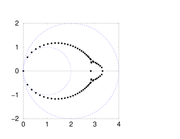
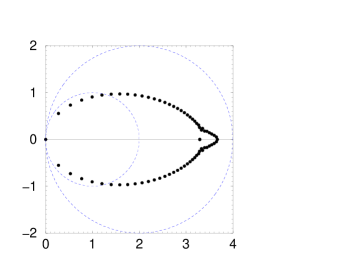
Figure 1: The spectrum of the FP Dirac operator $\Delta^{\rm\textstyle\scriptscriptstyle FP}$. The lattice size is $N=6$ and the number of iterations $n=5$; a) smooth background configuration with $Q^{\rm\textstyle\scriptscriptstyle FP}=1$; the range of the couplings considered in the action is $r_{g}=2$ (see subsection 4.1); the two circles represent the bounds on the spectrum, as explained in the text; b) as in a), but with $r_{g}=1$; c) and d) $r_{g}$=1 and background configuration with perturbation of size 0.5 and 1 respectively (still $Q^{\rm\textstyle\scriptscriptstyle FP}=1$).

Fig. 1 displays the spectrum of the FP Dirac operator on a $6^{2}$ lattice for background configurations with $Q^{\rm\textstyle\scriptscriptstyle FP}=1$. The Dirac operator has been obtained through 5 RG iterations. The deformation of the spectrum induced by the cut can be observed by comparing Figs. 1-a and 1-b, which refer to the two different cuts $r_{g}=2$ and $r_{g}=1$ respectively, in the case of a smooth background configuration. We see that for $r_{g}=2$ the bounds on the eigenvalues are well satisfied, while for $r_{g}=1$ a slight violation comes into play in the left edge of the spectrum due to the approximation of the sharp cut of the couplings. Comparison between Figs. 1-b and 1-c,d allows to evaluate the stability of the spectrum against perturbation of the background configuration, corresponding the two latter cases to a perturbation of the background configuration of size 0.5 and 1 respectively (the cut is always $r_{g}=1$). In all cases, except d, we find three real eigenvalues $\lambda_{\textstyle\scriptscriptstyle 0}<\lambda_{\textstyle\scriptscriptstyle 1}<\lambda_{\textstyle\scriptscriptstyle 2}$: the lowest one, $\lambda_{\textstyle\scriptscriptstyle 0}$ corresponds to the would be zero mode, see below; $\lambda_{\textstyle\scriptscriptstyle 1}$ is twofold degenerate. In the case d, where a strong perturbation of the background configuration is applied, the real eigenvalues are six, with no degeneracy. The higher real eigenvalues, lying on the right edge of the spectrum, are always decoupled from the infrared part of the spectrum, where the lowest real eigenvalue $\lambda_{\textstyle\scriptscriptstyle 0}$ is located.

It is interesting the comparison with the case of the (massless) Wilson operator, which has been studied recently in Ref. [35]; the eigenvalues fulfil in this case an additional symmetry [35], the reflection with respect to the point (2, 0) in the complex plane. For comparison with the FP case, we report in Fig. 2 the spectrum of the Wilson operator for the smooth configuration with topological charge one.

In Fig. 3 the evolution of the spectrum under the RG process starting from the Wilson operator is displayed, for $n=1,2,3$ and 4, in the case of the smooth configuration. We see that already for $n=1$ the spectrum has assumed the main features of its characteristic geometry, and only small changes take place thereafter; in particular, for $n=4$ the convergence to the final spectrum seems to be reached with good accuracy. It is also possible to observe the progressive decoupling of the two higher real eigenvalues $\lambda_{\textstyle\scriptscriptstyle 1}$ and $\lambda_{\textstyle\scriptscriptstyle 2}$, drifting towards higher values, from the lowest one $\lambda_{\textstyle\scriptscriptstyle 0}$, converging to zero.

5.2 Zero modes and index theorem

From the discussion of Sec. 2 we know that the FP Dirac operator must have zero modes in the topologically non trivial sectors, with definite chirality and satisfying the Index Theorem, Eq. (1), if the continuum topological charge is replaced by the FP topological charge $Q^{\rm\textstyle\scriptscriptstyle FP}$. In the Schwinger model the Vanishing Theorem (36) must also be true. As a consequence, in the case $Q^{\rm\textstyle\scriptscriptstyle FP}>0$, the FP Dirac operator should have $Q^{\rm\textstyle\scriptscriptstyle FP}$ zero modes with positive chirality. Since we do not attain exactly the FP, we do not expect exact zero modes. Rather, we expect that the $Q^{\rm\textstyle\scriptscriptstyle FP}$ lowest lying eigenvalues converge to zero when the number of iterations tends to infinity. Still, the cut of the couplings in the region $|x^{\prime}-x|>r_{g}$ can produce unwanted effects.

We start the discussion with the smooth configuration. In Table 3 we can see the eigenvalues of smallest modulo as a function of the number of iterations $i$. We report also the overall chirality of the zero modes (trace of $\gamma_{5}$ in the subspace of zero modes, $\sum_{v}(v,\gamma_{5}\,v)$), which should equal the FP topological charge of the background configuration. Notice that the eigenvalues are (within machine precision) real for $i=0$; this is in agreement with the observation [35] that eigenvectors with non-zero average chirality must have necessarily real eigenvalues. This is an exact statement, relying only on the hermiticity property of the fermion matrix (29), which is preserved by the RG procedure. The small numbers $O(10^{-6})$ found for the imaginary part of the eigenvalues for $i\geq 1$ are due to the approximation introduced when operating the matrix inversion in the recursion (the ultra-local approximation does not violate the hermiticity property). In accordance with the Index and Vanishing Theorem, in the case $Q^{\rm\textstyle\scriptscriptstyle FP}=1$ we find only one non-degenerate small real eigenvalue, while for $Q^{\rm\textstyle\scriptscriptstyle FP}=2$ the lowest lying eigenvalue is twofold degenerate. The real part of the eigenvalues converges towards zero when increasing the number of iterations; the law is roughly as $1/2^{i}$, as expected from the dimensional analysis of the lowest dimensional irrelevant operators. This law breaks down for $i=5$ in the case $r_{g}=1$, where we find numbers smaller than expected. The eigenvectors have in any case definite positive chirality, regardless to the number of iterations. In fact, this is already true for the starting Dirac operator, and the cut of the couplings seems not to be effective in this regard.

In conclusion, our results are consistent with the picture of a FP Dirac operator exactly verifying the Index Theorem, and being well approximated by ultra-local fermion matrices.

It is interesting to compare these results with those given by the Wilson operator, displayed in Table 4. Notice how the Index theorem is only asymptotically verified for $N\rightarrow\infty$, i.e., in the continuum limit.

The numbers of Table 5 have been obtained by adding a random perturbation of size $0.5$ to the smooth configurations previously considered (see also Table 6). Notice that the lowest lying eigenvalues are about twice larger than the corresponding for the smooth configuration. Again they decrease by a factor of about 2 after each iteration. Notice also that the random perturbation removes the degeneracy of the two lowest lying eigenvalues in the case $Q^{\rm\textstyle\scriptscriptstyle FP}=2$. Finally, we see that the chirality is no more perfect from the start, but already for $i=4$ it is compatible with 1 within our numerical accuracy.

5.3 The topological charge

The FP topological charge can be obtained directly from the FP Dirac operator through the formula (27). This relation could be useful for the calculations of topological quantities in unquenched QCD with the FP action, since it gives automatically a prescription for the FP topological charge, once a parametrization of the FP fermion matrix has been found. In our approach, we can check how accurately this relation is verified as the number of iterations of the FP equation is increased. The results are displayed in Table 7. We see that the difference with the FP topological charge is less than $14\%$ after $4$ iterations and less than $4\%$ after $5$ iterations with $r_{g}=1$ in the case $Q=1$. Moreover, the results are stable under the perturbation of the background configuration. With $r_{g}=2$ we observed only a slight improvement.

6 Conclusions

We have presented an explicit example which illustrates that it is possible to compute an ultra-local approximation of the FP Dirac operator which preserves up to a very good accuracy all the important properties of the exact FP operator. We showed by numerical computation that in the case of the Schwinger model it is a very good approximation to consider only couplings between fermions contained in the same size-two plaquette (translated in 4 dimensions: size-two hypercube). We have confined our work to the classical properties, like zero modes and their chirality, topological charge and the Index Theorem. We have checked these properties in the case of instanton solutions of the equation of motion and random perturbations around them. We believe, however, that the quantum properties of the FP action, like for example the non-renormalization of the pion mass, will also hold with similar accuracy. An indication of this is that another property derived from the GWR, namely the relation (27) between the FP Dirac operator and the topological charge of the background gauge configuration, holds within this same accuracy also when introducing quantum fluctuations around the classical instanton solutions. We are nevertheless conscious of the fact [36] that these mildly perturbed configurations are not representative of the whole MC set of configurations at thermal equilibrium.

Recently a great attention has been paid to the Index theorem on the lattice. The goal was to find some traces of it, either using the standard Wilson action [35, 36], some chiral improved version of it [37] or approximated solutions of the GW relation constructed from the overlap formalism [38]. In all these cases, the Index theorem seems to hold only in a probabilistic sense. We hope to have convinced the reader that the exact Index theorem of Ref. [20] holds very accurately even with an ultra-local approximation of the FP Dirac operator.

Our ultimate conclusion is therefore that a parametrization of the FP action, involving only very localized couplings, with good scaling properties should be possible. Moreover, following the suggestion by Hasenfratz and Niedermayer, one can use the freedom typically present in this kind of fits to enforce up to a very high precision the classical properties for some instanton-like smooth configurations. A parametrization of the FP action of the Schwinger model was already found in [39], but locality was not the first priority of the authors in that work. Really, this is urgent problem only in view of four dimensional theories.

We solved the FP equation by iterations. The analytical solution of the pure gauge part (this is an extra-bonus of the two dimensions) enabled us to concentrate the numerical effort in the fermion sector. Also the low dimensionality of the model was of great help, but still, it was not possible to make many iterations. With five we got a good precision. In four dimensions, however, memory-space and CPU-time problems are likely to be an obstacle to this naive iterative approach. Different strategies to solve the FP equation should be devised. A possibility to avoid extremely large lattices is to use, as in [39], a parametrization of the FP action from the very beginning, namely to solve the iteration equation in a finite space of couplings.

Acknowledgments.

We are indebted with P. Hasenfratz and F. Niedermayer for stimulating discussions and useful suggestions. The work received financial support from Fonds zur Förderung der Wissenschaftlichen Forschung in Österreich - Austria, project P11502-PHY (F.F.), and Ministerio de Educación y Cultura - Spain under grant PF-95-73193582 (V.L.).

Figure 2: The spectrum of the Wilson operator $\Delta^{\textstyle\scriptscriptstyle\rm W}$ on a $6^{2}$ lattice for the smooth background configuration with $Q^{\rm\textstyle\scriptscriptstyle FP}=1$.

Figure 3: The evolution under RG of the spectrum of the Dirac operator on a $6^{2}$ lattice starting from the Wilson discretization $\Delta^{\textstyle\scriptscriptstyle\rm W}$, for number of iterations $n=1$ (a), $n=2$ (b), $n=3$ (c), $n=4$ (d). The smooth background configuration has charge $Q^{\rm\textstyle\scriptscriptstyle FP}=1$ and $r_{g}=1$.

$Q=1$
	$r_{g}=1$				$r_{g}=2$
$i$	${\textstyle\rm Re}\,\lambda$	${\textstyle\rm Im}\,\lambda$	$\sum_{v}\,(v,\,\gamma_{5}v)$		${\textstyle\rm Re}\,\lambda$	${\textstyle\rm Im}\,\lambda$	$\sum_{v}\,(v,\,\gamma_{5}v)$
0	0.1240	6.0$\>\>10^{-16}$	1.0000		—	—	—
1	0.0778	1.4$\>\>10^{-7}$	1.0000		0.0611	$-3.7$$\>\>10^{-7}$	1.0000
2	0.0466	7.3$\>\>10^{-7}$	1.0000		0.0290	$-1.2$$\>\>10^{-6}$	1.0000
3	0.0250	$-1.3$$\>\>10^{-6}$	1.0000		0.0134	$-4.9$$\>\>10^{-6}$	1.0000
4	0.0101	6.4$\>\>10^{-6}$	1.0000		0.0065	9.6$\>\>10^{-7}$	1.0000
5	0.0017	$7.4$$\>\>10^{-9}$	1.0000		0.0039	$-5.2$$\>\>10^{-6}$	1.0000
$Q=2$
0	0.2441	$-3.0$$\>\>10^{-16}$	2.0000		—	—	—
1	0.1570	3.6$\>\>10^{-8}$	1.9998		0.1233	$-1.9$$\>\>10^{-6}$	2.0000
2	0.0960	8.7$\>\>10^{-7}$	1.9998		0.0598	$-3.5$$\>\>10^{-6}$	2.0000
3	0.0531	$-7.6$$\>\>10^{-7}$	1.9998		0.0281	$-6.8$$\>\>10^{-6}$	2.0000
4	0.0233	6.8$\>\>10^{-6}$	1.9998		0.0135	1.4$\>\>10^{-6}$	2.0000
5	0.0026	$-1.3$$\>\>10^{-5}$	2.0000

Table 3: The lowest lying eigenvalue and the chirality of the corresponding eigenvectors of the Dirac operator for a smooth background gauge configuration ($Q=1$ and $2$), for each number of iterations $i$. The lattice size is $N=6$. $r_{g}$ is the range over which the approximated action extends, see subsection 4.1.

$N$	${\textstyle\rm Re}\,\lambda$	${\textstyle\rm Im}\,\lambda$	$(v,\,\gamma_{5}v)$
4	0.3183	1.2$\>\>10^{-16}$	0.8258
6	0.1438	1.2$\>\>10^{-15}$	0.8372
8	0.0805	5.7$\>\>10^{-17}$	0.8678
10	0.0504	6.9$\>\>10^{-17}$	0.8909
12	0.0340	2.5$\>\>10^{-16}$	0.9073
14	0.0242	$-1.8$$\>\>10^{-16}$	0.9193
16	0.0180	$-4.9$$\>\>10^{-16}$	0.9284
18	0.0138	4.8$\>\>10^{-15}$	0.9357
20	0.0109	1.4$\>\>10^{-15}$	0.9415
22	0.0088	$-5.5$$\>\>10^{-15}$	0.9463
24	0.0073	3.6$\>\>10^{-15}$	0.9505

Table 4: The lowest lying eigenvalue and the chirality of the corresponding eigenvector of the Wilson Dirac operator on lattices of different sizes $N$, with the smooth background configuration having $Q=1$.

$Q=1$
	$r_{g}=1$				$r_{g}=2$
$i$	${\textstyle\rm Re}\,\lambda$	${\textstyle\rm Im}\,\lambda$	$(v,\,\gamma_{5}v)$		${\textstyle\rm Re}\,\lambda$	${\textstyle\rm Im}\,\lambda$	$(v,\,\gamma_{5}v)$
0	0.2109	$-1.0$$\>\>10^{-15}$	0.9739		—	—	—
1	0.1242	$-1.1$$\>\>10^{-5}$	0.9938		0.0966	5.4$\>\>10^{-7}$	0.9938
2	0.0797	$-9.9$$\>\>10^{-6}$	0.9980		0.0450	6.3$\>\>10^{-7}$	0.9985
3	0.0512	$-1.1$$\>\>10^{-5}$	0.9993		0.0204	$-7.1$$\>\>10^{-7}$	0.9997
4	0.0317	$-2.7$$\>\>10^{-6}$	0.9996		0.0092	3.6$\>\>10^{-6}$	1.0000
5	0.0184	$-2.0$$\>\>10^{-6}$	0.9997		0.0046	$-2.2$$\>\>10^{-6}$	1.0000
$Q=2$
0	0.2603	$-4.6$$\>\>10^{-16}$	0.9792		—	—	—
	0.3493	$-8.0$$\>\>10^{-16}$	0.9506		—	—	—
1	0.1589	2.5$\>\>10^{-6}$	0.9955		0.1249	$-8.2$$\>\>10^{-7}$	0.9957
	0.2150	$-4.7$$\>\>10^{-6}$	0.9884		0.1676	1.5$\>\>10^{-6}$	0.9909
2	0.0989	3.7$\>\>10^{-6}$	0.9986		0.0603	7.7$\>\>10^{-7}$	0.9989
	0.1371	$-8.3$$\>\>10^{-6}$	0.9960		0.0807	$-1.0$$\>\>10^{-6}$	0.9980
3	0.0583	6.9$\>\>10^{-7}$	0.9995		0.0377	$-1.2$$\>\>10^{-6}$	0.9996
	0.0850	$-9.4$$\>\>10^{-6}$	0.9984		0.0283	4.7$\>\>10^{-6}$	0.9998
4	0.0299	7.9$\>\>10^{-6}$	0.9998		0.0174	$-1.5$$\>\>10^{-7}$	1.0000
	0.0490	$-4.4$$\>\>10^{-6}$	0.9992		0.0133	3.5$\>\>10^{-6}$	1.0000

Table 5: The same as table 3 adding a random fluctuation of size $0.5$ to the smooth configuration.

$i$	${\textstyle\rm Re}\,\lambda$	${\textstyle\rm Im}\,\lambda$	$(v,\,\gamma_{5}v)$
0	0.3348	2.0$\>\>10^{-16}$	0.9282
1	0.1824	1.1$\>\>10^{-5}$	0.9869
2	0.1245	9.7$\>\>10^{-6}$	0.9963
3	0.0908	5.7$\>\>10^{-6}$	0.9986
4	0.0679	8.7$\>\>10^{-6}$	0.9990
5	0.0520	$-2.2$$\>\>10^{-6}$	0.9989

Table 6: The same as table 3 adding a random fluctuation of size $1$ to the smooth configuration. In this case $Q=1$ and $r_{g}=1$.

	$Q=1$				$Q=2$
$i$	smooth	Pert. 0.5	pert. 1		smooth	Pert. 0.5	Pert. 1
1	0.2289	0.2280	0.2118		0.4565	0.4498	0.4263
2	0.5114	0.5067	0.4906		1.0067	0.9954	0.9691
3	0.7223	0.7185	0.7100		1.4143	1.4020	1.3902
4	0.8668	0.8637	0.8663		1.6959	1.6839	1.6878
5	0.9631	0.9608	0.9740		1.8844	—	—

Table 7: The value of $-\frac{1}{2\kappa_{\rm\textstyle\scriptscriptstyle F}}\,{\rm tr}\,\left(\gamma_{5}\,\{\Delta^{\rm\scriptscriptstyle FP},\,R^{\rm\textstyle\scriptscriptstyle FP}\}\,\right)$ for the smooth configurations and perturbations around them; $N=6$ and $r_{g}=1$.

A Appendix

In this Appendix we solve explicitly the minimization problem  (40) when in the r.h.s. the Manton action is taken. The result will be $\alpha^{\rm\textstyle\scriptscriptstyle min}(\alpha^{\prime})$, and so $U_{\mu}^{\rm\textstyle\scriptscriptstyle min}(U^{\prime})=\exp(i\alpha_{\mu}^{\rm\textstyle\scriptscriptstyle min}(\alpha^{\prime}))$.

Of course, due to gauge invariance, the fine configuration $\alpha_{\mu}(x)$ solving Eq. (40) is not unique; indeed, an entire orbit of solutions exists, all related by gauge transformations not altering the fixed coarse configuration $\alpha_{\mu}^{\prime}(x_{b})$. It is possible to exploit this restricted freedom and fix the gauge in order to simplify the problem.

We (partially) fix the gauge by requiring:

$$\alpha^{\rm\textstyle\scriptscriptstyle min}_{\mu}(2x_{b})\;=\;\alpha^{\rm\textstyle\scriptscriptstyle min}_{\mu}(2x_{b}+\hat{\mu})\;\;,\;\;\;\;\;\;\;\;\;\mu=1,2\;\;.$$ (A.1)

In this gauge, the constraint:

$$[\,\alpha_{\mu}(2x_{b})+\alpha_{\mu}(2x_{b}+\hat{\mu})\,]\>({\rm mod}\;2\pi)\>=\>\alpha^{\prime}_{\mu}(x_{b})$$ (A.2)

has the solution:

$$\alpha^{\rm\textstyle\scriptscriptstyle min}_{\mu}(2x_{b})\>=\>\alpha^{\rm\textstyle\scriptscriptstyle min}_{\mu}(2x_{b}+\hat{\mu})\>=\>\frac{1}{2}\,\alpha_{\mu}^{\prime}(x_{b})\>+\>n_{\mu}(x_{b})\,\pi\;\;,$$ (A.3)

where $n_{\mu}(x_{b})$ can be 0 or $\pm 1$ (the sign depending on the sign of $\alpha_{\mu}^{\prime}(x_{b})$); exploiting the gauge freedom we can fix: $n_{\mu}(x_{b})=0$.

For a given lattice site of the blocked lattice $x_{b}$, we define the block of the sites of the fine lattice belonging to $x_{b}$ as: $\{x:\,x\,=\,2x_{b}+\lambda_{1}\hat{1}+\lambda_{2}\hat{2},\lambda_{\mu}=0,1,2\}$. We see that in our particular gauge, the condition (A.2) fixes the eight fine links lying on the border of the above defined blocks (Eq. (A.3)). As a consequence, the residual minimizing problem decouples in the various blocks; indeed the remaining degrees of freedom are the links internal to the blocks (four for each block), and links internal to different blocks do not communicate between themselves.

Minimization inside each block can be now trivially performed. Here gauge invariance can be again exploited by fixing:

$$\alpha^{\textstyle\scriptscriptstyle\rm min}_{\textstyle\scriptscriptstyle 1}(2x_{b}+\hat{2})\>=\>\alpha^{\textstyle\scriptscriptstyle\rm min}_{\textstyle\scriptscriptstyle 1}(2x_{b}+\hat{1}+\hat{2})\;\;.$$ (A.4)

The result is:

$$\alpha^{\rm\textstyle\scriptscriptstyle min}_{\textstyle\scriptscriptstyle 2}(2x_{b}+\hat{1}) = \frac{1}{4}(\alpha^{\prime}_{\textstyle\scriptscriptstyle 2}(x_{b})+\alpha^{\prime}_{\textstyle\scriptscriptstyle 2}(x_{b}+\hat{1}))\>+\>(n_{\textstyle\scriptscriptstyle 1}(x_{b})-n_{\textstyle\scriptscriptstyle 2}(x_{b}))\,\pi\;\;\;\;$$

$$\alpha^{\rm\textstyle\scriptscriptstyle min}_{\textstyle\scriptscriptstyle 1}(2x_{b}+\hat{2}) = \alpha^{\rm\textstyle\scriptscriptstyle min}_{\textstyle\scriptscriptstyle 1}(2x_{b}+\hat{1}+\hat{2})\>\>=$$

$$\frac{1}{4}(\alpha^{\prime}_{\textstyle\scriptscriptstyle 1}(x_{b})\!\!\!\! + \!\!\!\!\alpha^{\prime}_{\textstyle\scriptscriptstyle 1}(x_{b}+\hat{2}))\>+\>(n_{\textstyle\scriptscriptstyle 3}(x_{b})+n_{\textstyle\scriptscriptstyle 4}(x_{b})-n_{\textstyle\scriptscriptstyle 1}(x_{b})-n_{\textstyle\scriptscriptstyle 2}(x_{b}))\,\frac{\pi}{2}\;\;\;\;$$

$$\alpha^{\rm\textstyle\scriptscriptstyle min}_{\textstyle\scriptscriptstyle 2}(2x_{b}+\hat{1}+\hat{2}) = \frac{1}{4}(\alpha^{\prime}_{\textstyle\scriptscriptstyle 2}(x_{b})+\alpha^{\prime}_{\textstyle\scriptscriptstyle 2}(x_{b}+\hat{1}))\>+\>(n_{\textstyle\scriptscriptstyle 4}(x_{b})-n_{\textstyle\scriptscriptstyle 3}(x_{b}))\,\pi\;\;,\;$$ (A.5)

where the integer numbers $n_{i}(x_{b}),i=1,2,3,4$, are involved in the consistency conditions

$$F_{\textstyle\scriptscriptstyle 12}^{\rm\textstyle\scriptscriptstyle L}(2x_{b})-n_{\textstyle\scriptscriptstyle 1}(x_{b})\,2\pi\>\in\>(-\pi,\pi]\;\;,$$ (A.6)

and analogous relations respectively for $F_{\textstyle\scriptscriptstyle 12}^{\rm\textstyle\scriptscriptstyle L}(2x_{b}+\hat{1})$, $F_{\textstyle\scriptscriptstyle 12}^{\rm\textstyle\scriptscriptstyle L}(2x_{b}+\hat{1}+\hat{2})$ and $F_{\textstyle\scriptscriptstyle 12}^{\rm\textstyle\scriptscriptstyle L}(2x_{b}+\hat{2})$, where $F_{\textstyle\scriptscriptstyle 12}^{\rm\textstyle\scriptscriptstyle L}(x)$ is the lattice field tensor for the solving fine configuration given by Eqs. (A.3) and (A.5). For this solution, one has:

$$F_{\textstyle\scriptscriptstyle 12}^{\rm\textstyle\scriptscriptstyle L}(2x_{b})\>-\>n_{\textstyle\scriptscriptstyle 1}\,2\pi\>=\>F_{\textstyle\scriptscriptstyle 12}^{\rm\textstyle\scriptscriptstyle L}(2x_{b}+\hat{1})\>-\>n_{\textstyle\scriptscriptstyle 2}\,2\pi\>=\>F_{\textstyle\scriptscriptstyle 12}^{\rm\textstyle\scriptscriptstyle L}(2x_{b}+\hat{1}+\hat{2})\>-\>n_{\textstyle\scriptscriptstyle 3}\,2\pi\>=$$

$$F_{\textstyle\scriptscriptstyle 12}^{\rm\textstyle\scriptscriptstyle L}(2x_{b}+\hat{2})\>-\>n_{\textstyle\scriptscriptstyle 4}\,2\pi\>=\>\frac{1}{4}F_{\textstyle\scriptscriptstyle 12}^{{\rm\textstyle\scriptscriptstyle L}\,\prime}(x_{b})\>-\>(n_{\textstyle\scriptscriptstyle 1}+n_{\textstyle\scriptscriptstyle 2}+n_{\textstyle\scriptscriptstyle 3}+n_{\textstyle\scriptscriptstyle 4})\,\frac{\pi}{2}\;\;,\;\;\;\;\;\;\;\;\;\;$$ (A.7)

where we indicate with $F_{\textstyle\scriptscriptstyle 12}^{{\rm\textstyle\scriptscriptstyle L}\,\prime}(x_{b})$ the field tensor of the coarse configuration $\alpha^{\prime}(x_{b})$. Using the above relations, its is clear that the total action of the fine configuration, according to Manton’s definition, reads:

$$\frac{1}{2}\sum_{x}\,\left[\,F^{\rm\textstyle\scriptscriptstyle L}_{\textstyle\scriptscriptstyle 12}(x)\;({\rm mod}\,2\pi)\,\right]^{2}\>=\;\;\;\;\;\;\;\;\;\;\;\;\;\;\;\;\;\;\;\;\;\;\;\;\;\;\;\;\;\;\;$$

$$\frac{1}{8}\sum_{x_{b}}\,\left[\,F_{\textstyle\scriptscriptstyle 12}^{{\rm\textstyle\scriptscriptstyle L}\,\prime}(x_{b})-(n_{\textstyle\scriptscriptstyle 1}(x_{b})+n_{\textstyle\scriptscriptstyle 2}(x_{b})+n_{\textstyle\scriptscriptstyle 3}(x_{b})+n_{\textstyle\scriptscriptstyle 4}(x_{b}))\,2\pi\,\right]^{2}\;\;.$$ (A.8)

The absolute minimum of the r.h.s. of the above equation among variations of the $n_{i}(x_{b})$’s is given by:

$$S^{\min}\>=\>\frac{1}{8}\sum_{x_{b}}\,\left[\,F_{\textstyle\scriptscriptstyle 12}^{\rm\textstyle\scriptscriptstyle L\,\prime}(x_{b})\,{(\rm mod}\,2\pi)\,\right]^{2}\;\;.$$ (A.9)

Observe that the set of integer numbers realizing the absolute minimum (A.9) satisfy in particular the consistency relation (A.6) and the other three analogous relations for $F_{\textstyle\scriptscriptstyle 12}^{\rm\textstyle\scriptscriptstyle L}(2x_{b}+\hat{1})$, $F_{\textstyle\scriptscriptstyle 12}^{\rm\textstyle\scriptscriptstyle L}(2x_{b}+\hat{1}+\hat{2})$ and $F_{\textstyle\scriptscriptstyle 12}^{\rm\textstyle\scriptscriptstyle L}(2x_{b}+\hat{2})$. Eq. (A.9) is the Manton action for the coarse configuration, apart from a factor $1/4$, which renormalizes the coupling in a trivial way, $\beta\rightarrow\beta/4$.

For the fine minimizing configuration the following relation holds (see Eq. (A.7)):

$$F^{\rm\textstyle\scriptscriptstyle L}_{\textstyle\scriptscriptstyle 12}(x)\;({\rm mod}\,2\pi)\>=\>\frac{1}{4}\,\left[F^{\rm\textstyle\scriptscriptstyle L\prime}_{\textstyle\scriptscriptstyle 12}(x_{b})\;({\rm mod}\,2\pi)\right]\;,\;\;\;x=2x_{b}+\lambda_{\textstyle\scriptscriptstyle 1}\hat{1}+\lambda_{\textstyle\scriptscriptstyle 2}\hat{2},\;\lambda_{\mu}=0,1\;\;,$$ (A.10)

from which it is evident that the lattice topological charge operator (47) reproduces itself under the RG transformation.

References

- [1] M. Lüscher, Commun. Math. Phys. 85 (1982) 39.
- [2] P. di Vecchia, K. Fabricius, G.C. Rossi and G. Veneziano, Nucl. Phys. B192 (1981) 392; K. Ishikawa, G. Schierholz, H. Schneider and M. Teper, Phys. Lett. B128 (1983) 309.
- [3] M. Campostrini, A. Di Giacomo and H. Panagopoulos, Phys. Lett. B212, (1988) 206.
- [4] H.B. Nielsen and M. Ninomiya, Phys. Lett B105 (1981) 219; Nucl. Phys. B185 (1981) 20.
-
[5]
M. Atiyah and I.M. Singer, Ann. Math. 93 (1971) 139;
A.S. Schwarz, Phys. Lett. 67B (1977) 172; L. Brown, R. Carlitz and C. Lee, Phys. Rev. D16 (1977) 417. - [6] For a recent summary on perfect actions, see P. Hasenfratz, hep-lat/9709110; for a pedagogical introduction, see P. Hasenfratz, in the proceedings of the ’NATO ASI - Confinement, Duality and Non-perturbative Aspects of QCD’, 1997, Ed. P. van Baal, Plenum Press, to be published.
- [7] P. Hasenfratz and F. Niedermayer, Nucl. Phys. B414 (1994) 785.
- [8] F. Farchioni, P. Hasenfratz, F. Niedermayer, and A. Papa, Nucl. Phys. B454 (1995) 638.
- [9] F. Farchioni and V. Laliena, BUTP-97/24, hep-lat/9709040.
- [10] P. Hasenfratz and F. Niedermayer, Nucl. Phys. B507 (1997) 399.
- [11] T. DeGrand, A. Hasenfratz, P. Hasenfratz and F. Niedermayer, Nucl. Phys. B454 (1995) 587.
- [12] T. DeGrand, A. Hasenfratz, P. Hasenfratz and F. Niedermayer, Nucl. Phys. B454 (1995) 615.
- [13] A. Papa, Nucl. Phys. B478 (1996) 335.
- [14] A. Papa, hep-lat/9710091.
- [15] M. Blatter, R. Burkhalter, P. Hasenfratz and F. Niedermayer, Phys. Rev. D53 (1996) 923.
- [16] M. D’Elia, F. Farchioni and A. Papa, Phys. Rev. D55 (1997) 2274.
- [17] T. DeGrand, A. Hasenfratz, P. Hasenfratz, P. Kunszt and F. Niedermayer, Nucl. Phys. B53 (Proc. supp.) (1997) 942;
- [18] F. Niedermayer, Nucl. Phys. B (Proc. Suppl.) 53 (1997) 56; K. Orginos, W. Bietenholz, R. Brower, S. Chandrasekharan and U.-J. Wiese, hep-lat/9709100.
- [19] See the first reference in [6].
- [20] P. Hasenfratz, V. Laliena and F. Niedermayer, hep-lat/9801021.
- [21] P. Hasenfratz, hep-lat/9802007.
- [22] P.H. Ginsparg and K.G Wilson, Phys. Rev. D25 (1982) 2649.
- [23] M. Luescher, hep-lat/9802011.
- [24] H. Neuberger, hep-lat/9707022; hep-lat/9801031; R. Narayanan and H. Neuberger, Phys. Rev. Lett. 71 (1993) 3251; Nucl. Phys. B433 (1995) 305.
- [25] See the second reference in [6].
- [26] P. Kunszt, hep-lat/9706019.
- [27] P. van Baal, Comm. Math. Phys. 85 (1982) 529.
- [28] J. Kikis, Phys. Rev. D15 (1977) 2329; N.K. Nielsen, B. Schroer, Nucl. Phys. B127 (1977) 493; M.M Ansourian, Phys. Lett. B70 (1977) 301.
- [29] J. Smit and J.C. Vink, Nucl. Phys. B284 (1987) 234.
- [30] N.S. Manton Phys. Lett. B96 (1980) 328.
- [31] N.S. Manton, Ann. of Phys. 159 (1985) 220.
- [32] W. Bietenholz, R. Brower, S. Chandrasekharan and U.-J. Wiese, Phys. Lett. B407 (1997) 283.
- [33] P. de Forcrand, J.E. Hetrick, T. Takaishi and A.J. van der Sijs, hep–lat/9709104.
- [34] M. Kremer, A.S. Kronfeld, M.L. Laursen, G. Schierholz and U.-J. Wiese, Nucl. Phys. B305 (1988) 109; D.J.R. Pugh and M. Teper, Phys. Lett. B224 (1989) 159; M. Göckeler, A.S. Kronfeld, M.L. Laursen, G. Schierholz and U.-J. Wiese, Phys. Lett. B233 (1989) 192.
- [35] C.R. Gattringer, I. Hip and C.B. Lang, Nucl. Phys. B508 (1997) 329.
- [36] C.R. Gattringer, I. Hip and C.B. Lang, Phys. Lett. B409 (1997) 391.
- [37] P. Hernández, hep-lat/9801035.
- [38] R. Narayanan and H. Neuberger, Nucl. Phys. B443 (1995) 305; R. Narayanan and P. Vranas, Nucl. Phys. B506 (1997) 373; R. Narayanan and R. Singleton, hep-lat/9709014; R.G. Edwards, U.M. Heller, R. Naranayan and E.L. Singleton, hep-lat/9711029.
- [39] C.B. Lang and T.K. Pany, Nucl. Phys. B513 (1998) 645.