Abstract

Topology on the lattice is reviewed. In quenched QCD topological susceptibility $\chi$ is fully understood. The Witten-Veneziano mechanism for the $\eta^{\prime}$ mass is confirmed. The topological susceptibility drops to zero at the deconfining phase transition. Preliminary results are also presented for $\chi$ and $\chi^{\prime}$ in full QCD, and for the spin content of the proton. The only problem there is the difficulty of the usual Hybrid Monte Carlo algorithm to bring topology to equilibrium.

1 Introduction

Topology plays a fundamental role in QCD. The key equation is the $U_{A}(1)$ anomaly

$$\partial_{\mu}J_{\mu}^{5}=-2N_{f}Q(x)$$ (1)

where $J^{5}_{\mu}=\sum_{i=1}^{N_{f}}\overline{\psi}_{i}\gamma^{5}\gamma_{\mu}\psi_{i}$ is the singlet axial current, $N_{f}$ the number of light flavours and

$$Q(x)={g^{2}\over{64\pi^{2}}}F_{\mu\nu}^{a}F_{\rho\sigma}^{a}\epsilon_{\mu\nu\rho\sigma}$$ (2)

is the topological charge density. $Q(x)$ is related to the Chern current $K_{\mu}(x)$

$$\partial_{\mu}K_{\mu}(x)=Q(x)$$ (3)

with

$$K_{\mu}={g^{2}\over{16\pi^{2}}}\epsilon_{\mu\nu\rho\sigma}A^{a}_{\nu}\left(\partial_{\rho}A^{a}_{\sigma}-{1\over 3}gf^{abc}A^{b}_{\rho}A^{c}_{\sigma}\right)$$ (4)

and as a consequence $Q=\int Q(x)$ is an integer on smooth classical configurations with finite action. Eqs. (1-3) yield

$$\partial_{\mu}\left(J^{5}_{\mu}(x)+2N_{f}K_{\mu}(x)\right)=0$$ (5)

whence Ward identities can be derived. At the leading order in the $1/N_{c}$ expansion, ($N_{c}\longrightarrow\infty$, with $g^{2}N_{f}$ fixed), $Q(x)$ is zero, $U_{A}(1)$ is a symmetry and $\eta^{\prime}$ is its Goldstone particle, $m_{\eta^{\prime}}=0$. The anomaly acts as a perturbation and shifts the position of the pole from zero to the actual $\eta^{\prime}$ mass. From Eq.(5) by inserting the quark mass terms, the relation follows [1, 2]

$$\chi={{f_{\pi}^{2}}\over{2N_{f}}}\left(m_{\eta}^{2}+m_{\eta^{\prime}}^{2}-2m_{K}^{2}\right)$$ (6)

where $\chi$ is the topological susceptibility of the unperturbed vacuum $(1/N_{c}=0)$ defined as

$$\chi=\int\hbox{d}^{4}(x-y)\partial^{x}_{\mu}\partial^{y}_{\nu}\langle 0|T(K_{\mu}(x)K_{\nu}(y))|0\rangle_{\rm quenched}.$$ (7)

The subscript “quenched” indicates that the matrix element has to be computed on the ground state of the $1/N_{c}=0$ theory. In particular this implies that fermion loops, which are $O(g^{2}N_{f})$ are put to zero. Eq.(6) gives

$$\chi=(180\;\hbox{MeV})^{4}$$ (8)

which is expected to be valid within an order $O(1/N_{c})$ of accuracy. Eq.(6) is a peculiar equation relating physical quantities (masses, $f_{\pi}$, $N_{f}$) to $\chi$, which exists in an artificial $1/N_{c}=0$ world. Its verification, however, is a check of the validity of the expansion, which is a fundamental issue. Lattice is an ideal tool to produce this artificial world, and in particular the absence of fermions in it simplifies the numerical work. Eq.(7) uniquely fixes the prescription for the singularity in the product of operators $K_{\mu}(x)K_{\nu}(y)$ as $x\longrightarrow y$: $\delta$-like singularities disappear after integration and this uniquely determines $\chi$. Eq.(7) is a specific prescription for the notation

$$\chi=\int\hbox{d}^{4}x\langle 0|T(Q(x)Q(0))|0\rangle_{\rm quenched}.$$ (9)

When computing $\chi$ by any regularization scheme, like lattice, an appropriate subtraction must be performed to satisfy the prescription Eq.(7).

The behaviour of $\chi$ at finite temperature, and more specifically, at deconfinement, is an important key to understand the structure of QCD vacuum [3]

A regularized version of the operator $Q(x)$, $Q_{L}(x)$, can be defined on the lattice. There is a large arbitrariness in this definition, by terms of higher order in the lattice-spacing which go to zero in the continuum limit. In general $Q_{L}(x)$ will not be an exact divergence, so that a multiplicative renormalization $Z$ with respect to continuum can exist [4]. If $a$ is the lattice-spacing,

$$Q_{L}(x)=a^{4}ZQ(x)+O(a^{6}).$$ (10)

A lattice susceptibility $\chi_{L}$ is defined as

$$\chi_{L}=\sum_{x}\langle Q_{L}(x)Q_{L}(0)\rangle={{\langle Q_{L}^{2}\rangle}\over V}.$$ (11)

In general the definition (11) will not satisfy the prescription Eq. (7). It will be [5]

$$\chi_{L}=a^{4}Z^{2}\chi+M+O(a^{6})$$ (12)

where $M$ is a mixing with the continuum operators having dimension $\leq 4$ ($\overline{\beta}$ is the beta function)

$$M(\beta)=A(\beta)\langle{{\overline{\beta}(g)}\over g}F^{a}_{\mu\nu}F^{a}_{\mu\nu}\rangle a^{4}+P(\beta)\cdot 1.$$ (13)

From Eq.(12)

$$\chi={{\chi_{L}-M}\over{Z^{2}a^{4}}}.$$ (14)

$\chi_{L}$ is measured on the lattice numerically. $a^{4}$ is determined as usual by comparison to a physical quantity ($\rho$ mass, string tension); $M$ and $Z$ can be determined non-perturbatively by a procedure known as heating [6]. The idea is that classical configurations with known topological charge, can be dressed by quantum fluctuations without modifying the topological content since topological charge is difficult to change by the usual local Monte Carlo algorithms. $Z$ is determined by measuring the total charge $Q_{L}$ on a configuration with an instanton, where $Q=1$, Eq.(10). $M$ is determined from Eq.(12) by measuring $\chi_{L}$ on the sector $Q=0$, where as a consequence of Eq.(7), $\chi=0$.

In Eq.(14) $\chi_{L}$, $M$ and $Z$ strongly depend on the choice of $Q_{L}$, on the action and on the coupling constant $\beta=2N_{c}/g^{2}$. $a$ depends on the action and on $\beta$. $\chi$ must be independent of all these parameters. Fig. 1 shows $\chi$ for $SU(3)$ [7], determined for several $\beta$’s and by use of different operators: as visible in the figure $\chi=(175\pm 5$ MeV)⁴. For $SU(2)$ (Fig. 2) [8] $\chi$ is somewhat larger: $\chi=(198\pm 6$ MeV)⁴.

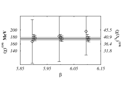
Figure 1: $\chi$ for $SU(3)$. Diamonds, circles and squares correspond to the 0, 1 and 2-smeared operators.

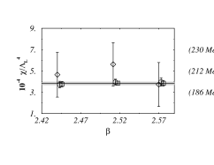
Figure 2: $\chi$ for $SU(2)$. Diamonds, circles and squares correspond to the 0, 1 and 2-smeared operators.

The determination by using the so-called geometrical method, if accompained by the appropriate subtraction, agrees with the other choices of $Q_{L}$.

Fig. 3 shows the behaviour of $\chi$ across deconfinement. The drop is stronger for $SU(3)$ than for $SU(2)$ [8].

Figure 3: $\chi$ across the deconfinement transition for $SU(2)$ (circles) and $SU(3)$ (squares).

2 Full QCD

By use of the same procedure described in the previous section, $\chi$ can be determined in full QCD. The expectation from the Ward identities is that

$$\chi\approx\langle\sum_{i=1}^{N_{f}}m_{i}\overline{\psi}_{i}\psi_{i}\rangle+O(m_{q}^{2}).$$ (15)

Our preliminary result, extracted from simulating at $\beta=5.35$ where $a=0.11(1)$ fm with 4 staggered fermions at $am=0.01$ is

$$\chi=(110\pm 8\;\hbox{MeV})^{4}$$ (16)

to be compared to the predicted value

$$\chi={m_{q}\over N_{f}}\langle\overline{\psi}\psi\rangle_{m=0}\sim(109\;\hbox{MeV})^{4}.$$ (17)

On the same sample of configurations we obtain for $\chi^{\prime}$ the preliminary value

$$\chi^{\prime}=258\pm 100\;\hbox{MeV}^{2}\;\;\;\;\hbox{or}\;\;\;\sqrt{\chi^{\prime}}=19\pm 4\;\hbox{MeV}$$ (18)

which is compatible with the value expected from sum rules [9] $\sqrt{\chi^{\prime}}=25\pm 3\;\hbox{MeV}$. However both these determinations are preliminary because of the effect shown in Fig. 4 where we display the history of the topological charge $Q$ along the Monte Carlo updating which produces the configurations [10]. In the updating algorithms used in quenched QCD (Metropolis, heat-bath) the topological charge has tipically $50-100$ steps of authocorrelation time. It thermalizes slowly with respect to local quantum fluctuations (and this is the basic property which allows the heating method for the measurement of $Z$ and $M$ as explained in section 1), but a thermalized sample of configurations can be prepared in a reasonable CPU time. The algorithm used with dynamical fermions, the hybrid Monte Carlo, performs very badly in that respect, as is visible from Fig. 4. The configurations there correspond to about 700 CPU hours of an APE Quadrics with 25 GFlop which is a huge time. Our sample has thus a much smaller number of independent configurations than shown in Fig. 4, and therefore the errors in the results given in Eqs. (16) and (18) are underestimated.

Figure 4: History of $Q$ in a Hybrid Monte Carlo run as a function of the molecular dynamic time $\tau$.

The same uncertainty affects our determination, on the same sample, of the spin content of the proton. The matrix element of $J^{5}_{\mu}$ between proton states can be parametrized as

$$\langle{\vec{p}^{\prime}},s^{\prime}|J^{5}_{\mu}|{\vec{p}},s\rangle=\overline{u}({\vec{p}^{\prime}},s^{\prime})\left(G_{1}(k^{2})\gamma_{\mu}\gamma^{5}-G_{2}(k^{2})\gamma^{5}k_{\mu}\right)u({\vec{p}},s)$$ (19)

with $k=p-p^{\prime}$. The form factor $G_{1}$ is related to the so-called spin content of the proton $\Delta\Sigma$, $G_{1}(0)=\Delta\Sigma$ where $\Delta\Sigma\equiv\Delta u+\Delta d+\Delta s$ is the contribution of the different quarks species to the spin of the proton. The naïve expectation would be $\Delta\Sigma\sim 0.7$. The value determined from the moments of the spin dependent structure functions of inelastic scattering of leptons on nucleons is much lower: $\Delta\Sigma=0.2(1)$. The lattice allows a determination of $\Delta\Sigma$ from first principles. One possible technique consists in the direct measurement of the matrix element (19). An alternative is to use the anomaly equation, which after taking the divergence of both sides of Eq.(19),

$$\langle{\vec{p}^{\prime}},s^{\prime}|Q|{\vec{p}},s\rangle = {m_{N}\over N_{f}}A(k^{2})\overline{u}({\vec{p}^{\prime}},s^{\prime})i\gamma^{5}u({\vec{p}},s)$$ (20)

$$A(k^{2}) = G_{1}(k^{2})+{k^{2}\over m_{N}}G_{2}(k^{2}).$$ (21)

As $k\longrightarrow 0$ Eq.(21) determines $G_{1}(0)$, unless $G_{2}(k^{2})$ has a pole at $k^{2}=0$ and this is the case in the quenched approximation but not in full QCD. Eq. (20) gives thus $\Delta\Sigma$ in terms of the matrix element $\langle{\vec{p}^{\prime}},s^{\prime}|Q|{\vec{p}},s\rangle$, which can be measured on the lattice. In principle the lattice operator $Q_{L}$ would mix with $\partial_{\mu}J^{5}_{\mu}(x)$ and $\overline{\psi}\gamma^{5}\psi$, but this mixing, as well as the small anomalous dimension of $Q$ can be neglected [11]. Our preliminary value is $\Delta\Sigma=0.04(4)$. Here again the error could be larger and in any case the value is preliminary, due to the bad sampling of topology in our ensemble of configurations.

3 Conclusions

Measurement of the topological susceptibility $\chi$ on the lattice is fully under control. For quenched $SU(3)$ the value is in good agreement with the prediction of [1, 2]. $\chi$ drops to zero at the deconfining transition. Preliminary determinations of $\chi^{\prime}$ in full QCD agree with sum rules. The spin content of the proton is at hand. The practical problem is the thermalization of topology on the lattice. Our huge sample of configurations is not thermalized with respect to it. This creates in principle a problem for the lattice determination of any quantity: a priori, indeed, it is not known how it could depend on the topological sector and therefore if the ensemble is biased with respect to topology, this could affect the result in an impredictable way. Solutions of this numerical problem are currently under study.

References

- [1] E. Witten, Nucl. Phys. B156 (1979) 269.
- [2] G. Veneziano, Nucl. Phys. B159 (1979) 213.
- [3] E. Shuryak, Comments Nucl. Part. Phys. 21 (1994) 235.
- [4] M. Campostrini, A. Di Giacomo, H. Panagopoulos, Phys. Lett. B212 (1988) 206.
- [5] M. Campostrini, A. Di Giacomo, H. Panagopoulos, E. Vicari, Nucl. Phys. B329 (1990) 683.
- [6] A. Di Giacomo, E. Vicari, Phys. Lett. B275 (1992) 429.
- [7] B. Allés, M. D’Elia, A. Di Giacomo, Nucl. Phys. B494 (1997) 281.
- [8] B. Allés, M. D’Elia, A. Di Giacomo, Phys. Lett. B412 (1997) 119.
- [9] S. Narison, G. M. Shore, G. Veneziano, Nucl. Phys. B433 (1995) 209.
- [10] B. Allés, G. Boyd, M. D’Elia, A. Di Giacomo, E. Vicari, Phys. Lett. B389 (1996) 107.
- [11] B. Allés, A. Di Giacomo, H. Panagopoulos, E. Vicari, Phys. Lett. B350 (1995) 70.