Numerical Study of the
Fundamental Modular Region
in the Minimal Landau Gauge

Abstract

We study numerically the so-called fundamental modular region $\Lambda$, a region free of Gribov copies, in the minimal Landau gauge for pure $SU(2)$ lattice gauge theory. To this end we evaluate the influence of Gribov copies on several quantities — such as the smallest eigenvalue of the Faddeev-Popov matrix, the third and the fourth derivatives of the minimizing function, and the so-called horizon function — which are used to characterize the region $\Lambda$. Simulations are done at four different values of the coupling: $\beta=0\mbox{,}\,0.8\mbox{,}\,1.6\mbox{,}\,2.7\,$, and for volumes up to $16^{4}$. We find that typical (thermalized and gauge-fixed) configurations, including those belonging to the region $\Lambda$, lie very close to the Gribov horizon $\partial\Omega$, and are characterized, in the limit of large lattice volume, by a negative-definite horizon tensor.

1 Introduction

Gauge theories, being invariant under local gauge transformations, are systems with redundant dynamical variables, which do not represent true dynamical degrees of freedom. The objects of interest are not the gauge fields themselves, but rather the classes (orbits) of gauge-related fields. The elimination of such redundant gauge degrees of freedom is essential for understanding and extracting physical information from these theories. This is usually done by introducing a gauge-fixing condition which determines a representative gauge field on each orbit. In reference [1] Gribov showed that Coulomb and Landau gauge-fixing conditions do not fix the gauge fields uniquely, i.e. there are many gauge-equivalent configurations satisfying the Coulomb or Landau transversality condition. These Gribov copies do not affect perturbative calculations, but their elimination could play a crucial role for non-perturbative features of gauge theories. Gribov’s result was generalized by Singer [2] to the case of a generic compact semi-simple non-abelian Lie group. In this work the author considered continuous gauge fixing, and boundary conditions (i.e. value of the gauge fields at infinity) such that the euclidean space-time is compactified to the four-dimensional sphere $S^{4}$. A similar analysis was done by Killingback [3] for the case of periodic boundary conditions (i.e. the four-dimensional torus $T^{4}$), which are the boundary conditions usually employed in lattice gauge theory.

A possible solution to the problem of Gribov copies is to restrict the functional integral to a subset of the gauge-field space, the fundamental modular region $\Lambda$, which is the set of absolute minima of a Morse function on the gauge orbits [4, 5]. In the so-called minimal Landau gauge this Morse function is defined as

$${\cal E}_{A}[g]\,\equiv\,\|\,A^{(g)}\,\|^{2}\,\equiv\,\frac{1}{2}\,\sum_{\mu\mbox{,}\,a}\,\int\,d^{d}x\,\left\{\,\left[\,A_{\mu}^{(g)}\,\right]^{a}(x)\,\right\}^{2}\;\mbox{.}$$ (1)

It has been proven [5, 6, 7, 8] that, with this choice of the Morse function, every orbit intersects the interior of the fundamental modular region once and only once, i.e. in the interior of $\Lambda$ the absolute minima are non-degenerate and there are no Gribov copies. However, on the boundary of the fundamental modular region there are degenerate absolute minima, and only when they have been identified can we obtain a region truly free of Gribov copies [5, 8].

The problem of Gribov copies is also present in the lattice regularization of gauge theories [9, 10]. Although this formulation does not require gauge fixing, due to asymptotic freedom, the continuum limit is the weak-coupling limit, and a weak-coupling expansion requires gauge fixing. Thus, gauge-dependent quantities are usually introduced on the lattice, and Gribov copies have to be taken into account in lattice gauge theory as well.

A fundamental modular region can be defined also on the lattice. In this case, for the minimal Landau gauge, we consider the absolute minima of the functional

$${\cal E}_{U}[g]\;\equiv\;\frac{1}{8\,V}\sum_{x}\sum_{\mu}\,\mathop{\rm Tr}\nolimits\,\left[\,1\!\!\!\bot\,-\,g(x)\;U_{\mu}(x)\;g^{\dagger}(x+e_{\mu})\,\right]\;\mbox{,}$$ (2)

which is the lattice analogue of the Morse function ${\cal E}_{A}[g]$ used in the continuum [see eq. (1)]. Since the gauge orbit is a compact manifold on a finite lattice, this functional is bounded and the existence of an absolute minimum for ${\cal E}_{U}$ follows immediately. Let us notice that the functional ${\cal E}_{U}[g]$ can be rewritten [12] as the quadratic form

$${\cal E}_{U}[g]\,=\,\frac{1}{8\,V}\sum_{x}\,g(x)\,\cdot\,\left(\,\nabla_{U}\,g\,\right)(x)\;\mbox{,}$$ (3)

where

$$\left(\,\nabla_{U}\,g\,\right)(x)\;=\,\sum_{\mu}\,\left[\,2\,g^{\dagger}(x)\,-\,U_{\mu}(x)\;g^{\dagger}(x+e_{\mu})\;-\;U_{\mu}^{\dagger}(x-ae_{\mu})\;g^{\dagger}(x-e_{\mu})\,\right]$$ (4)

is the gauge-covariant Laplacian. The minimization of a quadratic form is a standard and simple problem if the variables are elements of a linear space [13]. In our case, however, these variables are $SU(2)$ matrices (i.e. 4-dimensional unit vectors), and due to this non-linearity the numerical search for the absolute minimum becomes highly non-trivial.

Most of the properties proved in the continuum for the fundamental modular region can be extended to the lattice case [14, 15]. In particular, an explicit example of degenerate absolute minima on the boundary of $\Lambda$ is given in reference [14].

In this work we want to characterize the fundamental modular region by evaluating numerically diagnostic quantities (see Section 3) at relative and absolute minima. To date, relatively few studies [10, 11, 16] have been done in order to analyze the influence of Gribov copies (Gribov noise) on some lattice quantities. However, these numerical studies have never tried to characterize the “geometry” of the orbit space. We know general properties of the fundamental modular region, and we know particular cases in which this region can be studied analytically [5, 6, 7, 8, 14, 15, 17]. On the contrary, we do not know what happens in numerical simulations. This work aims at filling this gap, and at providing information about the “localization” in the gauge-field space of a typical thermalized gauge-fixed configuration. Preliminary results have been reported in [18].

2 Lattice Landau Gauge-Fixing Condition

In this section we analyze in more detail the lattice Landau gauge-fixing condition. Let us recall that this gauge condition is imposed by minimizing the functional ${\cal E}_{U}$, defined in eq. (2), with respect to the variables $\{g(x)\}$, keeping the thermalized configuration $\{U_{\mu}(x)\}$ fixed.

We consider a one-parameter subgroup $g(\tau;x)$ of $SU(2)$ defined by

$$g(\tau;x)\equiv\exp\left[\;i\,\tau\,\vec{\mbox{$\gamma$}}(x)\cdot\vec{\mbox{$\sigma$}}\;\right]\;\mbox{;}$$ (5)

here the parameter $\tau$ is a real number, $\vec{\mbox{$\gamma$}}(x)$ is a three-dimensional real vector, and the components of $\vec{\mbox{$\sigma$}}$ are the three Pauli matrices. Then the functional ${\cal E}_{U}$, defined in eq. (2), can be regarded as a function of the parameter $\tau$, and its first derivative — with respect to $\tau$ and at $\tau=0$ — is given by the well-known expression

$${\cal E}^{{}^{\prime}}(0)\,=\,\frac{1}{4\,V}\,\sum_{x}\,\sum_{a}\,\gamma^{a}(x)\,\left(\nabla\cdot A^{\left(g\right)}\right)^{a}(x)\;\mbox{,}$$ (6)

where

$$\left(\nabla\cdot A\right)^{a}(x)\equiv\sum_{\mu}\,A_{\mu}^{a}(x)-A_{\mu}^{a}(x-e_{\mu})$$ (7)

is the lattice divergence of the gluon field $\,A_{\mu}^{a}(x)\,$. If $\{U_{\mu}\left(x\right)\}$ is a stationary point of ${\cal E}(\tau)$ at $\tau=0$ then we have ${\cal E}^{{}^{\prime}}(0)=0$ for every $\{\gamma^{a}(x)\}$. This implies

$$\left(\nabla\cdot A\right)^{a}(x)=0$$ (8)

for any $x$ and $a$, which is the lattice formulation of the usual Landau gauge-fixing condition in the continuum.

Still considering the one-parameter subgroup defined in eq. (5), we can evaluate the second derivative of ${\cal E}(\tau)$. Following references [14, 15] one can check that

$${\cal E}^{{}^{\prime\prime}}(0) = \frac{1}{4\,V}\sum_{x\mbox{,}\,y}\,\sum_{a\mbox{,}\,b}\,\gamma^{a}(x)\,{\cal M}_{U}^{a\,b}(x\mbox{,}y)\,\gamma^{b}(y)$$ (10)

$$\equiv \,\frac{1}{4\,V}\sum_{x}\,\sum_{\mu\mbox{,}\,a}\,\biggl{\{}\Bigl{[}\,\gamma^{a}(x+e_{\mu})\,-\,\gamma^{a}(x)\,\Bigr{]}^{2}\,U_{\mu}^{0}(x)$$

$$\,+\,\sum_{b\mbox{,}\,c}\,\epsilon^{abc}\,\Bigl{[}\,\gamma^{a}(x+e_{\mu})\,-\,\gamma^{a}(x)\,\Bigr{]}\,\Bigl{[}\,\gamma^{b}(x+e_{\mu})\,+\,\gamma^{b}(x)\,\Bigr{]}\,A^{c}_{\mu}(x)\biggl{\}}\;\mbox{,}$$

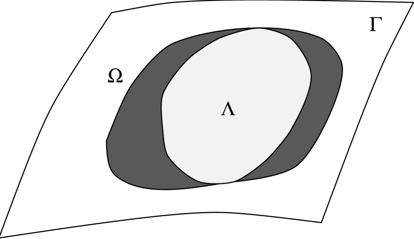
Figure 1:  The plane of the figure represents the hyperplane $\Gamma$ of transverse configurations ($\nabla\cdot A=0$). It contains the Gribov region $\Omega$ defined in eq. (11), and the fundamental modular region $\Lambda$. Note that parts of the boundaries $\partial\Omega$ and $\partial\Lambda$ are in common.

where ${\cal M}_{U}^{a\,b}(x\mbox{,}y)$ is the lattice Faddeev-Popov matrix and $\epsilon^{abc}$ is the complete anti-symmetric tensor. It is clear that this second derivative is null if the vector $\gamma^{a}(x)$ is constant, i.e. the Faddeev-Popov matrix has a trivial null eigenvalue corresponding to a constant eigenvector. From eq. (10) we obtain that, if $\{U_{\mu}\left(x\right)\}$ is a local minimum of ${\cal E}(\tau)$ at $\tau=0$, then the matrix ${\cal M}_{U}$ is positive definite (in the subspace orthogonal to the space of constant vectors). This implies that any local minimum of the functional ${\cal E}_{U}$ belongs to the region (see Figure 1)

$$\Omega\equiv\left\{\,A\,:\,\nabla\cdot A\,=\,0\mbox{,}\,\,{\cal M}_{U}\,\geq\,0\,\right\}\;\mbox{.}$$ (11)

This region was introduced by Gribov [1] in the attempt of getting rid of spurious gauge copies. It is delimited by the so-called first Gribov horizon $\partial\Omega$, i.e. the set of configurations for which the smallest nontrivial eigenvalue $\lambda_{min}$ of the Faddeev-Popov matrix is zero. Clearly the Gribov region $\Omega$ includes the fundamental modular region $\Lambda$. However, there are points — the so-called singular boundary points [5, 8, 14, 15, 17] — on the boundary of $\Lambda$ which are also on the boundary of $\Omega$ (see Figure 1). A typical example are degenerate absolute minima of the Morse function for which the degeneracy is continuous. In fact, as said in the Introduction, all the degenerate absolute minima are found on the boundary of the fundamental modular region. In the case of a continuous degeneracy, the Faddeev-Popov operator must have a zero eigenvalue, i.e. these minima are also on the boundary of $\Omega$. An explicit example of singular boundary points on the lattice has been found by Zwanziger (see [14, Appendix E]).

Finally, we can evaluate the third and fourth derivatives of ${\cal E}(\tau)$ with respect to $\tau$, at $\tau=0$. Following again [14, 15] we obtain

$${\cal E}^{{}^{\prime\prime\prime}}(0) = \frac{3}{4\,V}\sum_{x}\,\biggl{\{}\left[\,{\vec{\mbox{$\gamma$}}}^{2}(x+e_{\mu})\,-\,{\vec{\mbox{$\gamma$}}}^{2}(x)\,\right]\,\sum_{\mu\mbox{,}\,a}\,\Bigl{[}\,\gamma^{a}(x+e_{\mu})\,+\,\gamma^{a}(x)\,\Bigr{]}\,A^{a}_{\mu}(x)\,\biggl{\}}$$ (12)

$$\qquad\,\,\,\,\,\,\,-\,\frac{1}{V}\sum_{x}\,\biggl{\{}\,{\vec{\mbox{$\gamma$}}}^{2}(x)\,\sum_{a}\,\Bigl{[}\,\gamma^{a}(x)\,\left(\nabla\cdot A\right)^{a}(x)\,\Bigr{]}\,\biggl{\}}$$

and

$${\cal E}^{{}^{\prime\prime\prime\prime}}(0) = \frac{3}{4\,V}\sum_{x}\,\sum_{\mu}\,\biggl{\{}\Bigl{[}\,{\vec{\mbox{$\gamma$}}}^{2}(x+e_{\mu})\,-\,{\vec{\mbox{$\gamma$}}}^{2}(x)\,\Bigr{]}^{2}\,U_{\mu}^{0}(x)\,\Biggl{\}}$$ (13)

$$\quad-\,\frac{1}{V}\sum_{x\mbox{,}\,y}\,\biggl{\{}\,{\vec{\mbox{$\gamma$}}}^{2}(x)\,\sum_{a\mbox{,}\,b}\,\Bigl{[}\,\gamma^{a}(x)\,{\cal M}_{U}^{a\,b}(x\mbox{,}\,y)\,\gamma^{b}(y)\,\Bigr{]}\,\biggl{\}}\;\mbox{.}$$

3 Characterization of the Fundamental Modular Region

In order to characterize the “localization” of the gauge-fixed configuration in the hyperplane $\Gamma$ of transverse configurations ($\nabla\cdot A=0$; see Figure 1), we consider the smallest nonzero eigenvalue $\lambda_{min}$ of the Faddeev-Popov matrix ${\cal M}_{U}$, and its corresponding eigenvector $\omega^{a}_{min}(x)$, i.e. we solve the eigenvalue problem

$$\sum_{y}\,\sum_{b}\,{\cal M}_{U}^{a\,b}(x\mbox{,}\,y)\,\omega^{b}_{min}(y)\,=\,\lambda_{min}\,\omega^{a}_{min}(x)\;\mbox{.}$$ (14)

As already said, the matrix ${\cal M}_{U}$ has a trivial null eigenvalue corresponding to a constant eigenvector. Therefore, this equation has to be solved in the subspace orthogonal to constant vectors, namely the eigenvector $\omega^{a}_{min}(x)$ should satisfy the relation $\sum_{x}\,\omega^{a}_{min}(x)\,=\,0$. As for the eigenvalue $\lambda_{min}$, we know that it is positive, since any local minimum of ${\cal E}_{U}$ belongs to $\Omega$. Moreover, for the vacuum configuration $U_{\mu}(x)\,=\,1\!\!\!\bot\,$ (which also belongs to $\Omega$ and to $\Lambda$), the Faddeev-Popov matrix is simply (minus) the lattice Laplacian. Therefore, in this case, the value of $\lambda_{min}$ is given by

$$\lambda_{Lap}\,=\,4\sin^{2}\left(\,\pi/N\,\right)\;\mbox{,}$$ (15)

where $N$ is the lattice size. Finally, this eigenvalue goes to zero as the first Gribov horizon $\partial\Omega$ is approached. So, the value of $\lambda_{min}$ can be interpreted as a sort of distance between the minimum and $\partial\Omega$, and we may test whether its value is largest (in average) for the absolute minimum.

After we have evaluated the eigenvector $\omega^{a}_{min}(x)$, we can set $\gamma^{a}(x)\,=\,\omega^{a}_{min}(x)$ in the one-parameter subgroup defined in eq. (5). Then, if $\{\,U_{\mu}(x)\,\}$ is the configuration which minimizes the functional ${\cal E}_{U}$, we can study the behavior of the minimizing functional near the minimum using the gauge transformation generated by this one-parameter subgroup. More exactly, we can analyze its behavior along the “direction” of $\omega^{a}_{min}(x)$, i.e. along the direction for which the rate of increase of the functional ${\cal E}_{U}$ is smallest. To this end we expand ${\cal E}(\tau)$ in powers of $\tau$ around the minimum, i.e. around $\tau=0$. We then write

$${\cal E}(\tau)\,=\,{\cal E}(0)\,+\,\frac{\tau^{2}}{2}\,\left[\,{\cal E}^{{}^{\prime\prime}}(0)\,+\,\frac{\tau}{3}\,{\cal E}^{{}^{\prime\prime\prime}}(0)\,+\,\frac{\tau^{2}}{12}\,{\cal E}^{{}^{\prime\prime\prime\prime}}(0)\,\right]\,+\,\ldots\;\mbox{,}$$ (16)

where the derivatives of ${\cal E}(\tau)$ [see equations (10), (12) and (13)] are evaluated with $\gamma^{a}(x)\,=\,\omega^{a}_{min}(x)$, and the eigenvector $\omega^{a}_{min}(x)$ is normalized to one. We can now define the ratio

$$r\,\equiv\,\frac{\left[\,{\cal E}^{{}^{\prime\prime\prime}}(0)\,\right]^{2}}{{\cal E}^{{}^{\prime\prime}}(0)\,{\cal E}^{{}^{\prime\prime\prime\prime}}(0)}\;\mbox{,}$$ (17)

which is independent of the scale $\tau$, and rewrite equation (16) as

$${\cal E}(\tau)\,=\,{\cal E}(0)\,+\,\frac{\tau^{2}\,{\cal E}^{{}^{\prime\prime}}(0)}{2}\,\left[\,1\,+\,\frac{1}{3}\,\frac{\tau\,{\cal E}^{{}^{\prime\prime\prime}}(0)}{{\cal E}^{{}^{\prime\prime}}(0)}\,+\,\frac{1}{12\,r}\,\left(\,\frac{\tau\,{\cal E}^{{}^{\prime\prime\prime}}(0)}{{\cal E}^{{}^{\prime\prime}}(0)}\,\right)^{2}\,\right]\,+\,\ldots\;\;\mbox{.}$$ (18)

If we make the change of variables $x\equiv\tau\,{\cal E}^{{}^{\prime\prime\prime}}(0)/{\cal E}^{{}^{\prime\prime}}(0)$, then it is clear that the shape of the minimizing function around its minimum is fixed by the value of the ratio $r$. As an example, in Figure 2, we show the behavior of $\,{\cal E}(\tau)\,-\,{\cal E}(0)\,$ for six different values of the ratio $r$. Let us notice that, for $r>8/3$, there are Gribov copies of the minimum at $\tau=0$; in particular, there is a maximum, which does not belong to the Gribov region $\Omega$, and a second minimum, which is an example of a Gribov copy inside the first Gribov horizon $\partial\Omega$. Thus, we expect a value of $r$ smaller (in average) for the absolute minimum than for a generic relative minimum. Let us also notice that plots in Figure 2 are related to the bifurcation process described in reference [5]. In that case the author was following a stationary point of the minimizing function, while moving from inside to outside the region $\Omega$. Here, on the contrary, we sit at the minimum at $\tau=0$ and look at its surroundings for different values of the ratio $r$. We note that changing the value of $r$ is equivalent to moving this minimum inside the region $\Omega$.

If we set $\gamma^{a}(x)\,=\,\omega^{a}_{min}(x)$, and $\omega^{a}_{min}(x)$ is normalized to $1$, then from formulae (10) and (14) we obtain $\lambda_{min}\,=\,4\,V\,{\cal E}^{{}^{\prime\prime}}(0)$. In our simulations we evaluate the eigenvalue $\lambda_{min}$, the third and fourth derivatives of the minimizing function, and the ratio $r$.

Recently Zwanziger proposed [14, 15] a modification of the $SU(N)$-Yang-Mills action which effectively constrains the functional integral to the fundamental modular region $\Lambda$ in minimal Landau gauge. This effective action is given by

$$S_{eff}[U]\,=\,\beta\,S_{W}[U]+\alpha\,H[U]\;\mbox{,}$$ (19)

where $\beta\,S_{W}[U]$ is the standard Wilson action, $\alpha$ is a new thermodynamic parameter and $H[U]$ is the so-called horizon function defined as

$$H[U]\,\equiv\,\frac{1}{12}\,\sum_{\mu\mbox{,}\,a}\,H_{\mu\,a\mbox{,}\,\mu\,a}[U]\;\mbox{.}$$ (20)

Here $H_{\mu\,a\mbox{,}\,\nu\,b}[U]$ is the horizon tensor given by

$$H_{\mu\,a\mbox{,}\,\nu\,b}[U]\equiv\sum_{x\mbox{,}\,y}\,\sum_{c\mbox{,}\,d}\,\biggl{\{}\,B^{c}_{\mu\,a}(x)\,\left(\,{\cal M}_{U}^{-1}\,\right)^{c\,d}(x\mbox{,}\,y)\,B^{d}_{\nu\,b}(y)\,\biggl{\}}\,-\,\delta_{\mu\,\nu}\,\delta_{a\,b}\,\sum_{x}\,U_{\mu}^{0}(x)$$ (21)

and

$$B^{c}_{\mu\,a}(x)\equiv\delta^{c}_{a}\,\left[\,U^{0}_{\mu}(x)\,-\,U^{0}_{\mu}(x-ae_{\mu})\,\right]\,+\,\epsilon^{\phantom{a}bc}_{a}\left[\,A^{b}_{\mu}(x)\,+\,A^{b}_{\mu}(x-ae_{\mu})\,\right]\;\mbox{.}$$ (22)

With this new action the standard Yang-Mills theory is recovered (in the infinite-volume limit) only when the thermodynamic parameter $\alpha$ has the critical value $\alpha_{cr}$ fixed by the so-called horizon condition

$$-\alpha_{cr}^{-1}\,=\,\lim_{V\to\infty}\frac{1}{V}\,\langle\,H[U]\,\rangle\;\mbox{.}$$ (23)

For the vacuum configuration $U_{\mu}(x)\,=\,1\!\!\!\bot\,$ we obtain $B^{c}_{\mu\,a}(x)=0$, and therefore the horizon tensor is diagonal and equal to $-\,\delta_{\mu\,\nu}\,\delta_{a\,b}\,V$. On the contrary, at the first Gribov horizon $\partial\Omega$, the term containing the inverse of the Faddeev-Popov matrix blows up, i.e. both the horizon tensor and the horizon function are positive and become larger and larger as we approach $\partial\Omega$. In particular, points on the boundary of $\Omega$ where the horizon function is infinite can be explicitly exhibited [19]. However, the horizon function is not necessarily infinite for all configurations on the boundary of $\Omega$. In fact we can rewrite this function as [15]

$$H[U]\,=\,\frac{1}{12}\,\sum_{\mu\mbox{,}\,a}\,\sum_{n}\,\frac{1}{\lambda_{n}}\,\left[\,\sum_{x\mbox{,}\,c}\,B^{c}_{\mu\,a}(x)\,\omega_{n}^{c}(x)\,\right]^{2}\,-\,\frac{1}{4}\,\sum_{x}\,\sum_{\mu}\,U_{\mu}^{0}(x)\;\mbox{,}$$ (24)

where $\lambda_{n}$ and $\omega_{n}^{c}(x)$ are, respectively, the eigenvalues and the corresponding normalized eigenvectors of the Faddeev-Popov matrix ${\cal M}_{U}$. Then, for the so-called degenerate gauge orbits [15], one obtains that the absolute minimum is degenerate, namely it is on the common boundaries of $\Lambda$ and $\Omega$, and that the term of the horizon function which is proportional to $1/\lambda_{min}$ is of the indeterminate form $0/0$. In the infinite-volume limit the horizon tensor is expected [15] to be negative-definite inside the fundamental modular region $\Lambda$, and to vanish on its boundary. In the same limit, the measure should get concentrated [15] on a region where the horizon tensor per unit volume $h_{\mu\,a\mbox{,}\,\nu\,b}(U)$ is equal to zero. It is interesting to recall that the condition $h(U)=0$, where $h(U)$ is the horizon function per unit volume, is satisfied for all transverse configurations on a finite lattice with free boundary conditions [20]. However, this result is not sufficient to make lattices of this kind free of Gribov copies [21]. In order to test these conjectures, we evaluate the 12 eigenvalues of the horizon tensor (per unit volume) and the horizon function (also per unit volume). We also consider the average projection (per unit volume) of the $B^{c}_{\mu\,a}(x)$ vectors on the eigenvector $\omega_{min}^{c}(x)$, i.e.

$${\cal P}\equiv\frac{1}{12\,V}\,\sum_{\mu\mbox{,}\,a}\,\left[\,\sum_{x\mbox{,}\,c}\,B^{c}_{\mu\,a}(x)\,\omega_{min}^{c}(x)\,\right]^{2}\;\mbox{,}$$ (25)

and the contribution ${\cal P}/\lambda_{min}$ to the horizon function $h$ from this eigenvector [see formulae (24) and (25)]. Finally, we evaluate the largest and the smallest (both in absolute value) non-diagonal elements of the matrix ${\widetilde{h}}_{\mu\,a\mbox{,}\,\nu\,b}\equiv 12\,h_{\mu\,a\mbox{,}\,\nu\,b}$, and the average over its non-diagonal elements defined as

$$\left(\frac{1}{132}\,\sum_{i\mbox{,}\,j\mbox{;}\,i\neq j}\,{\widetilde{h}}_{ij}^{2}\,\right)^{1/2}\;\mbox{.}$$ (26)

4 Numerical Simulations

In order to evaluate the horizon tensor, and the horizon function, we have to invert the Faddeev-Popov matrix ${\cal M}_{U}$ [see equations (20) and (21)]. This matrix is rather large and sparse, and has an eigenvalue zero corresponding to constant modes. This means that it cannot be inverted directly. Nevertheless, this inversion can be done by using a standard conjugate-gradient (CG) method, provided that we work in the subspace orthogonal to constant vectors (see refences [11, 18, 22]). In particular, we have to impose that the source and the initial guess for the CG-method have zero constant mode. In our case the source is given by one of the (twelve) vectors $B^{c}_{\mu\,a}(x)$ defined in eq. (22). Thus, before inverting the matrix ${\cal M}_{U}$ we have to impose the condition

$$\sum_{x}\,B^{c}_{\mu\,a}(x)\,=\,0\;\mbox{.}$$ (27)

The evaluation of the smallest nonzero eigenvalue of ${\cal M}_{U}^{a\,b}(x\mbox{,}\,y)$ can be done using the routine that inverts this matrix. To this end let us consider the vector

$$\omega^{a}_{m}(x)\,\equiv\,\sum_{y}\,\sum_{b}\,\left(\,{\cal M}_{U}^{-m}\,\right)^{a\,b}(x\mbox{,}\,y)\,\omega^{b}(y)\;\mbox{,}$$ (28)

where $\omega^{b}(y)$ is a randomly chosen vector such that $\sum_{y}\,\omega^{b}(y)\,=\,0$. Then, in the limit of large $m$, we have

$$\omega^{a}_{m}(x)\,=\,\,c\,\lambda^{-m}_{min}\,\omega^{a}_{min}(x)\,+\,\ldots\;\;\mbox{,}$$ (29)

where $c$ is an unknown constant. This implies

$$\lambda_{min}\,=\,\frac{\omega^{a}_{m}(x)}{\omega^{a}_{m+1}(x)}$$ (30)

for any $a$ and $x$, and $\omega^{a}_{min}(x)$ is given by the vector $\omega^{a}_{m}(x)$ normalized to $1$. There are of course more sophisticated algorithms to evaluate eigenvalues and eigenvectors of a matrix. However, for this case, this simple method converges very fast and is easy to be implemented, since it uses the same conjugate-gradient routine used to evaluate the horizon tensor.

We consider, for each quantity, two different averages:

• Average (indicated as “am”) only on the supposed absolute minima.

• Average (indicated as “fc”) only on the first gauge-fixed gauge copy generated for each thermalized configuration. This is the result that we would obtain if Gribov copies were not considered.

If the result obtained from these two averages are systematically different for a given quantity, we can say that the existence of Gribov copies introduces a bias (Gribov noise) on the numerical evaluation of that quantity.

The parameters used for the simulations can be found in [11, Table 1]. However, in this paper, configurations at $\beta=1.6$ and with lattice volume $V=24^{4}$ were not analyzed. Our runs were started with a randomly chosen configuration. Details about thermalization (using hybrid overrelaxation) and gauge-fixing (using stochastic overrelaxation) can be found in references [11, 18, 23]. Computations were performed on several IBM RS-6000/250–340 workstations at New York University.

5 Results

In Table 1 we report the data for the ratio $\lambda_{min}/\lambda_{Lap}$, the third and the fourth derivatives of the minimizing function, and the ratio $r$ defined in eq. (17). For the third derivative we consider the absolute value since this quantity is negative for about $50\%$ of the configurations. The fourth derivative, on the contrary, is always positive, with very few exceptions at $\beta=2.7$ and small lattice volumes.

Our results are consistent with the conjectures discussed in Section 3: the value of $\lambda_{min}$ (respectively $r$) is larger (smaller), in average, for the absolute minima (average “am”). On the contrary, Gribov noise is not observable for the third and fourth derivatives of the minimizing function. Thus the Gribov noise for the ratio $r$ is entirely due to the Gribov noise of the eigenvalue $\lambda_{min}$. It is also interesting to observe that, for $\beta$ in the strong-coupling regime, $\lambda_{min}$ is down by a factor approximately $40-60$ with respect to the lowest nonzero eigenvalue $\lambda_{Lap}$ of the negative of the lattice Laplacian. (At $\beta=2.7$ this ratio is still about $6.5$.) This indicates that typical (thermalized and gauge-fixed) configurations, including those that are absolute minima, lie very close to the Gribov horizon $\partial\Omega$, where $\lambda_{min}=0$. Recall that the fundamental modular region $\Lambda$ is included in the Gribov region $\Omega$. Consequently we conclude that a typical configuration in $\Lambda$ lies close to its boundary $\partial\Lambda$, and where this boundary in turn lies close to $\partial\Omega$.

As for the quantity $r$, from Table 1 we observe that (where the statistics are good) $r$ is quite small, even though typical configurations lie near the boundary of the Gribov region $\partial\Omega$, as indicated by the remarkable smallness of $\lambda_{min}=4\,V\,{\cal E}^{{}^{\prime\prime}}(0)$. At a generic point of $\partial\Omega$ we have ${\cal E}^{{}^{\prime\prime\prime}}(0)\neq 0$, so $r=\infty$. However, at those points of $\partial\Omega$ that are also points of $\partial\Lambda$, we have ${\cal E}^{{}^{\prime\prime\prime}}(0)=0$ (see references [6, 14, 15]). The smallness of $r$ for relative (as well as absolute) minima is consistent with the hypothesis that also for typical configurations that are relative minima the boundary $\partial\Lambda$ lies close by. Note that whereas the gauge orbit is tangent to $\Gamma\,(\partial\cdot A=0)$ on a generic point of $\partial\Omega$, it is also tangent to $\partial\Omega$ at the common points of $\partial\Lambda$ and $\partial\Omega$ [6, 14, 15].

In Table 2 we report the data for the horizon function $h$, the contribution ${\cal P}/\lambda_{min}$ to the horizon function, and the minimizing function ${\cal E}_{U}$. Finally, in Table 3, we show the values for the smallest and the largest eigenvalues of the horizon tensor ${\widetilde{h}}_{a\,\mu\mbox{,}\,b\,\nu}$, and the average over its non-diagonal elements, as defined in eq. (26).

From our data there is evidence of Gribov noise for $h$ and for the eigenvalues of the horizon tensor: these quantities, in fact, are smaller at the absolute minima. Moreover, the horizon tensor is closer to a diagonal matrix at the absolute minima. On the contrary there is no evidence of Gribov noise for the quantity ${\cal P}$ defined in eq. (25). This suggests that the Gribov noise for ${\cal P}/\lambda_{min}$, a quantity which contributes to the value of the horizon function, is due to the eigenvalue $\lambda_{min}$. Note that ${\cal E}_{U}-1$ contributes to the horizon function $h$ also [see formulae (2) and (24)], and that ${\cal E}_{U}$ is (by definition) smallest at the absolute minimum. However, the Gribov noise for $h$ is much larger than the Gribov noise of ${\cal E}_{U}$ and ${\cal P}/\lambda_{min}$, i.e. it is probably due to Gribov noise for all the eigenvalues of the Faddeev-Popov matrix.

As for the volume dependence, it seems that the horizon tensor becomes closer and closer to a diagonal matrix as the lattice size increases (at fixed $\beta$). On the contrary, the value of the horizon function seems almost independent of the volume, while ${\cal P}$ and ${\cal P}/\lambda_{min}$ decrease with $V$. It is also evident that, at large enough volume, the horizon tensor is negative-definite. However, for small lattice volumes we find positive eigenvalues of the horizon tensor. We have also found, again at small values of $V$, a few configurations with a positive value for the horizon function $h$, even though $h$ is always negative in average, and its value approaches $-1$ (the value on the vacuum) as $\beta$ increases.

6 Conclusions

Our data show Gribov noise for quantities related to the Faddeev-Popov matrix, such as the eigenvalue $\lambda_{min}$ and the horizon tensor. This is in agreement with the result obtained in reference [11], in which Gribov noise has been observed for the ghost propagator. In all cases, the effect is small but clearly detectable for the values of $\beta$ in the strong-coupling region. The fact that this noise is not observable at $\beta=2.7$ seems to us to be related only to the small volumes considered here. Of course this hypothesis should be checked numerically. This is, at the moment, beyond the limits of our computational resources.

As for the “localization” in the gauge-field space of a typical (thermalized and gauge-fixed) configuration, the smallness of $\lambda_{min}$ and $r$ suggest that these configurations are always close to the common boundary of the Gribov region $\Omega$ and the fundamental modular region $\Lambda$. This is the case for relative as well as for absolute minima of the minimizing function. Moreover, in the limit of large lattice volume, only the region

$${\widetilde{\Omega}}\equiv\left\{\,A\,:\,A\in\Omega\mbox{,}\,\,H_{\mu\,a\mbox{,}\,\nu\,b}[U]\,<\,0\,\right\}$$ (31)

seems to contribute to the evaluated expectation values. Thus our results support the conjectures [15] that, in the limit of large lattice volume, the horizon tensor is negative-definite inside the fundamental modular region, and that the measure should get concentrated on the common boundary of $\Omega$ and $\Lambda$.

Figure 2:  Plot of $\,{\cal E}(\tau)\,-\,{\cal E}(0)\,$ as a function of $\tau$ for six different values of the ratio $r$ [see equations (17) and (18)]. For each value of $r$, the values for ${\cal E}^{{}^{\prime\prime}}(0)$ and ${\cal E}^{{}^{\prime\prime\prime}}(0)$, and the scale on the $y$ axis have been chosen “ad hoc” in order to emphasize the differences between the various cases. Recall that we are sitting at the minimum at $\tau=0$.

$\beta$	$N$	$aver$	$\lambda_{min}/\lambda_{Lap}$	$4\,V\,|{\cal E}_{U}^{{}^{\prime\prime\prime}}|$	$4\,V\,{\cal E}_{U}^{{}^{\prime\prime\prime\prime}}$	$r$
$0.0$	$4$	am	$0.0251(0.0005)$	$0.014028(0.000615)$	$0.08571(0.00259)$	$0.083(0.006)$
$0.0$	$4$	fc	$0.0230(0.0005)$	$0.015851(0.000654)$	$0.08960(0.00262)$	$0.124(0.010)$
$0.0$	$6$	am	$0.0204(0.0006)$	$0.005050(0.000369)$	$0.03441(0.00179)$	$0.084(0.015)$
$0.0$	$6$	fc	$0.0167(0.0005)$	$0.004918(0.000413)$	$0.02910(0.00159)$	$0.107(0.018)$
$0.0$	$8$	am	$0.0186(0.0006)$	$0.003719(0.000282)$	$0.02287(0.00144)$	$0.117(0.015)$
$0.0$	$8$	fc	$0.0162(0.0005)$	$0.003424(0.000236)$	$0.01954(0.00143)$	$0.141(0.020)$
$0.0$	$10$	am	$0.0169(0.0007)$	$0.003025(0.000384)$	$0.02435(0.00281)$	$0.140(0.026)$
$0.0$	$10$	fc	$0.0155(0.0007)$	$0.002912(0.000455)$	$0.01798(0.00232)$	$0.205(0.044)$
$0.0$	$12$	am	$0.0178(0.0008)$	$0.002056(0.000267)$	$0.01205(0.00110)$	$0.155(0.050)$
$0.0$	$12$	fc	$0.0163(0.0007)$	$0.002466(0.000400)$	$0.01565(0.00208)$	$0.230(0.083)$
$0.0$	$14$	am	$0.0199(0.0017)$	$0.002303(0.000484)$	$0.01685(0.00325)$	$0.218(0.078)$
$0.0$	$14$	fc	$0.0139(0.0010)$	$0.001605(0.000269)$	$0.01598(0.00349)$	$0.108(0.028)$
$0.0$	$16$	am	$0.0174(0.0018)$	$0.002259(0.000631)$	$0.01925(0.00835)$	$0.250(0.103)$
$0.0$	$16$	fc	$0.0157(0.0013)$	$0.003042(0.000873)$	$0.01267(0.00274)$	$0.453(0.240)$
$0.8$	$8$	am	$0.0238(0.0006)$	$0.004682(0.000541)$	$0.02340(0.00232)$	$0.165(0.035)$
$0.8$	$8$	fc	$0.0187(0.0006)$	$0.003929(0.000312)$	$0.01935(0.00127)$	$0.173(0.025)$
$0.8$	$12$	am	$0.0229(0.0015)$	$0.002674(0.000635)$	$0.01197(0.00376)$	$0.215(0.068)$
$0.8$	$12$	fc	$0.0178(0.0020)$	$0.002434(0.000478)$	$0.01582(0.00457)$	$0.245(0.083)$
$0.8$	$16$	am	$0.0257(0.0033)$	$0.002092(0.000652)$	$0.01576(0.00802)$	$0.140(0.052)$
$0.8$	$16$	fc	$0.0182(0.0030)$	$0.005938(0.004303)$	$0.02002(0.00875)$	$3.734(3.600)$
$1.6$	$8$	am	$0.0356(0.0013)$	$0.003807(0.000461)$	$0.01391(0.00132)$	$0.091(0.016)$
$1.6$	$8$	fc	$0.0277(0.0012)$	$0.004054(0.000513)$	$0.01569(0.00144)$	$0.205(0.061)$
$1.6$	$16$	am	$0.0289(0.0026)$	$0.003869(0.001529)$	$0.01001(0.00341)$	$0.764(0.427)$
$1.6$	$16$	fc	$0.0294(0.0022)$	$0.003136(0.001060)$	$0.01143(0.00296)$	$0.547(0.300)$
$2.7$	$8$	am	$0.1563(0.0051)$	$0.000568(0.000024)$	$0.00027(0.00002)$	$0.033(0.004)$
$2.7$	$8$	fc	$0.1552(0.0051)$	$0.000576(0.000026)$	$0.00028(0.00002)$	$0.036(0.004)$
$2.7$	$12$	am	$0.1476(0.0069)$	$0.000144(0.000018)$	$0.00008(0.00003)$	$0.030(0.005)$
$2.7$	$12$	fc	$0.1471(0.0069)$	$0.000157(0.000019)$	$0.00008(0.00003)$	$0.032(0.005)$
$2.7$	$16$	am	$0.1492(0.0084)$	$0.000063(0.000008)$	$0.00004(0.00003)$	$0.026(0.004)$
$2.7$	$16$	fc	$0.1476(0.0085)$	$0.000070(0.000011)$	$0.00006(0.00003)$	$0.027(0.004)$

Table 1:  The ratio between the smallest nonzero eigenvalue $\lambda_{min}$ of the Faddeev-Popov matrix and the smallest nonzero eigenvalue $\lambda_{Lap}$ of (minus) the lattice Laplacian [see eq. (15)], the absolute value of the third derivative and the fourth derivative of the minimizing function ${\cal E}_{U}$ [see formulae (12) and (13)], and the ratio $r$ defined in eq. (17). The derivatives of the minimizing function are multiplied by $4\,V$, where $V$ is the lattice volume. Two different types of statistics are considered: am = absolute minimum, and fc = first copy. Error bars (in brackets) are one standard deviation.

$\beta$	$N$	$aver$	$h$	${\cal P}/\lambda_{min}$	${\cal E}_{U}$
$0.0$	$4$	am	$-0.1046(0.0038)$	$0.0461(0.0022)$	$0.37810(0.00019)$
$0.0$	$4$	fc	$-0.0940(0.0043)$	$0.0515(0.0023)$	$0.37841(0.00019)$
$0.0$	$6$	am	$-0.1377(0.0026)$	$0.0206(0.0015)$	$0.37285(0.00012)$
$0.0$	$6$	fc	$-0.1286(0.0025)$	$0.0241(0.0015)$	$0.37328(0.00012)$
$0.0$	$8$	am	$-0.1388(0.0032)$	$0.0126(0.0014)$	$0.37151(0.00006)$
$0.0$	$8$	fc	$-0.1333(0.0018)$	$0.0117(0.0006)$	$0.37193(0.00006)$
$0.0$	$10$	am	$-0.1410(0.0011)$	$0.0071(0.0005)$	$0.37117(0.00006)$
$0.0$	$10$	fc	$-0.1328(0.0013)$	$0.0083(0.0008)$	$0.37151(0.00006)$
$0.0$	$12$	am	$-0.1392(0.0008)$	$0.0047(0.0004)$	$0.37116(0.00005)$
$0.0$	$12$	fc	$-0.1342(0.0009)$	$0.0049(0.0004)$	$0.37141(0.00005)$
$0.0$	$14$	am	$-0.1387(0.0015)$	$0.0027(0.0005)$	$0.37127(0.00007)$
$0.0$	$14$	fc	$-0.1317(0.0012)$	$0.0043(0.0006)$	$0.37148(0.00006)$
$0.0$	$16$	am	$-0.1359(0.0012)$	$0.0029(0.0005)$	$0.37133(0.00009)$
$0.0$	$16$	fc	$-0.1327(0.0018)$	$0.0032(0.0004)$	$0.37150(0.00008)$
$0.8$	$8$	am	$-0.1618(0.0024)$	$0.0144(0.0009)$	$0.32771(0.00008)$
$0.8$	$8$	fc	$-0.1434(0.0025)$	$0.0175(0.0010)$	$0.32815(0.00008)$
$0.8$	$12$	am	$-0.1559(0.0019)$	$0.0049(0.0006)$	$0.32737(0.00013)$
$0.8$	$12$	fc	$-0.1445(0.0040)$	$0.0101(0.0030)$	$0.32770(0.00013)$
$0.8$	$16$	am	$-0.1557(0.0019)$	$0.0022(0.0006)$	$0.32720(0.00013)$
$0.8$	$16$	fc	$-0.1479(0.0012)$	$0.0037(0.0006)$	$0.32740(0.00012)$
$1.6$	$8$	am	$-0.1994(0.0025)$	$0.0181(0.0013)$	$0.26763(0.00015)$
$1.6$	$8$	fc	$-0.1764(0.0047)$	$0.0291(0.0034)$	$0.26797(0.00016)$
$1.6$	$16$	am	$-0.1838(0.0027)$	$0.0057(0.0009)$	$0.26643(0.00010)$
$1.6$	$16$	fc	$-0.1810(0.0021)$	$0.0046(0.0008)$	$0.26670(0.00011)$
$2.7$	$8$	am	$-0.4961(0.0476)$	$0.1378(0.0234)$	$0.11122(0.00040)$
$2.7$	$8$	fc	$-0.4878(0.0482)$	$0.1436(0.0236)$	$0.11128(0.00040)$
$2.7$	$12$	am	$-0.5824(0.0164)$	$0.0789(0.0128)$	$0.10101(0.00024)$
$2.7$	$12$	fc	$-0.5759(0.0172)$	$0.0835(0.0133)$	$0.10104(0.00024)$
$2.7$	$16$	am	$-0.5710(0.0214)$	$0.0596(0.0096)$	$0.09821(0.00016)$
$2.7$	$16$	fc	$-0.5764(0.0176)$	$0.0474(0.0047)$	$0.09825(0.00016)$

Table 2:  The horizon function (per unit volume) $h\equiv H/V$ [see eq. (20)], the contribution ${\cal P}/\lambda_{min}$ to the horizon function $h$ from the eigenvector $\omega_{min}^{c}(x)$ [see formulae (24) and (25)], and the minimizing function ${\cal E}_{U}$ defined in eq. (2). Two different types of statistics are considered: am = absolute minimum, and fc = first copy. Error bars (in brackets) are one standard deviation.

$\beta$	$N$	$aver$	smallest eigen.	largest eigen.	aver. NDE
$0.0$	$4$	am	$-0.3039(0.0018)$	$0.4544(0.0316)$	$0.0613(0.0018)$
$0.0$	$4$	fc	$-0.3015(0.0019)$	$0.5243(0.0348)$	$0.0665(0.0020)$
$0.0$	$6$	am	$-0.2419(0.0014)$	$0.1295(0.0220)$	$0.0303(0.0013)$
$0.0$	$6$	fc	$-0.2394(0.0015)$	$0.1493(0.0192)$	$0.0340(0.0013)$
$0.0$	$8$	am	$-0.2105(0.0010)$	$0.0485(0.0320)$	$0.0195(0.0012)$
$0.0$	$8$	fc	$-0.2052(0.0010)$	$0.0346(0.0134)$	$0.0190(0.0005)$
$0.0$	$10$	am	$-0.1907(0.0009)$	$-0.0427(0.0065)$	$0.0123(0.0004)$
$0.0$	$10$	fc	$-0.1860(0.0010)$	$-0.0124(0.0098)$	$0.0139(0.0007)$
$0.0$	$12$	am	$-0.1769(0.0007)$	$-0.0694(0.0052)$	$0.0090(0.0003)$
$0.0$	$12$	fc	$-0.1737(0.0008)$	$-0.0628(0.0043)$	$0.0093(0.0003)$
$0.0$	$14$	am	$-0.1684(0.0011)$	$-0.0893(0.0063)$	$0.0067(0.0004)$
$0.0$	$14$	fc	$-0.1635(0.0011)$	$-0.0716(0.0062)$	$0.0076(0.0004)$
$0.0$	$16$	am	$-0.1603(0.0012)$	$-0.0922(0.0051)$	$0.0056(0.0003)$
$0.0$	$16$	fc	$-0.1569(0.0020)$	$-0.0887(0.0051)$	$0.0057(0.0003)$
$0.8$	$8$	am	$-0.2456(0.0013)$	$0.0209(0.0146)$	$0.0226(0.0007)$
$0.8$	$8$	fc	$-0.2362(0.0014)$	$0.0811(0.0162)$	$0.0261(0.0008)$
$0.8$	$12$	am	$-0.2035(0.0020)$	$-0.0708(0.0075)$	$0.0110(0.0005)$
$0.8$	$12$	fc	$-0.1976(0.0013)$	$-0.0132(0.0355)$	$0.0151(0.0027)$
$0.8$	$16$	am	$-0.1847(0.0013)$	$-0.1158(0.0054)$	$0.0061(0.0004)$
$0.8$	$16$	fc	$-0.1793(0.0015)$	$-0.0927(0.0048)$	$0.0073(0.0003)$
$1.6$	$8$	am	$-0.3158(0.0017)$	$0.0571(0.0153)$	$0.0306(0.0010)$
$1.6$	$8$	fc	$-0.3076(0.0019)$	$0.1985(0.0409)$	$0.0405(0.0030)$
$1.6$	$16$	am	$-0.2285(0.0025)$	$-0.1055(0.0124)$	$0.0110(0.0006)$
$1.6$	$16$	fc	$-0.2264(0.0017)$	$-0.1107(0.0069)$	$0.0104(0.0006)$
$2.7$	$8$	am	$-0.7818(0.0022)$	$1.7496(0.5495)$	$0.1412(0.0220)$
$2.7$	$8$	fc	$-0.7812(0.0024)$	$1.8130(0.5550)$	$0.1465(0.0222)$
$2.7$	$12$	am	$-0.7577(0.0017)$	$0.4859(0.1653)$	$0.0888(0.0126)$
$2.7$	$12$	fc	$-0.7565(0.0019)$	$0.5242(0.1705)$	$0.0910(0.0129)$
$2.7$	$16$	am	$-0.7303(0.0029)$	$0.2794(0.1947)$	$0.0708(0.0096)$
$2.7$	$16$	fc	$-0.7269(0.0038)$	$0.0821(0.1000)$	$0.0599(0.0047)$

Table 3:  The smallest and the largest eigenvalues of the matrix ${\widetilde{h}}_{\mu\,a\mbox{,}\,\nu\,b}\equiv 12\,H_{\mu\,a\mbox{,}\,\nu\,b}/V$ [see eq. (21)], and the average of its non-diagonal elements [see eq. (26)]. Two different types of statistics are considered: am = absolute minimum, and fc = first copy. Error bars (in brackets) are one standard deviation.

References

- [1] V.N.Gribov, Nucl.Phys. B139 (1978) 1.
- [2] I.M.Singer, Commun.Math.Phys. 60 (1978) 7.
- [3] T.P.Killingback, Phys.Lett. B138 (1984) 87.
- [4] J.Milnor, Morse Theory (Princeton University Press, Princeton NJ, 1963); J.Fuchs, M.G. Schmidt and C. Schweigert, Nucl.Phys. B426 (1994) 107.
- [5] P. van Baal, Nucl.Phys. B369 (1992) 259.
- [6] M.A.Semenov-Tyan-Shanskii and V.A.Franke, Zapiski Nauchnykh Seminarov Leningradskogo Otdeleniya Matematicheskogo Instituta im. V.A.Steklova AN SSSR 120 (1982) 159 [English translation: Journ.Sov.Math. 34 (1986) 1999].
- [7] G.Dell’Antonio and D.Zwanziger, Commun.Math.Phys. 138 (1991) 291.
- [8] P. van Baal, Nucl.Phys. B417 (1994) 215; P. van Baal, Global Issues in Gauge Fixing, hep-th/9511119, published in the Proceeding of the QCD Workshop, Trento (Italy) 1995.
- [9] E.Marinari, C.Parrinello and R.Ricci, Nucl.Phys. B362 (1991) 487; Ph. de Forcrand et al., Nucl.Phys. B (Proc. Suppl.) 20 (1991) 194; J.E.Mandula and M.C.Ogilvie, Phys.Rev. D41 (1990) 2586; J.E.Hetrick et al., Nucl.Phys. B (Proc. Suppl.) 26 (1992) 432; P.Marenzoni and P.Rossi, Phys.Lett. B311 (1993) 219; A.Nakamura and M.Mizutani, Vistas in Astronomy 37 (1993) 305.
- [10] Ph. de Forcrand and J.E.Hetrick, Nucl.Phys. B (Proc. Suppl.) 42 (1995) 861.
- [11] A.Cucchieri, Gribov Copies in the Minimal Landau Gauge: the Influence on Gluon and Ghost Propagators, hep-lat/9705005, ZiF-MS-16/97 preprint, to appear in Nucl.Phys. B.
- [12] M.Grabenstein, Analysis and Development of Stochastic Multigri Methods in Lattice Field Theory, Ph.D. thesis (Universität Hamburg), hep-lat/9401024.
- [13] See for example W.H.Press et al., Numerical Recipes (Cambridge University Press, Cambridge, 1992, second edition).
- [14] D.Zwanziger, Nucl.Phys. B378 (1992) 525.
- [15] D.Zwanziger, Nucl.Phys. B412 (1994) 657.
- [16] S.Hioki et al., Phys.Lett. B271 (1991) 201; A.Nakamura and M.Plewnia, Phys.Lett. B255 (1991) 274; M.L.Paciello et al., Phys.Lett. B289 (1992) 405; M.L.Paciello et al., Phys.Lett. B341 (1994) 341; V.G.Bornyakov et al., Nucl.Phys. B (Proc. Suppl.) 34 (1994) 802; U.M.Heller, F.Karsch and J.Rank, Phys.Lett. B355 (1995) 511; G.S.Bali et al., Nucl.Phys. B (Proc. Suppl.) 42 (1995) 852; L.Conti et al., Phys.Lett. B373 (1996) 164; G.S.Bali et al., Phys.Rev. D54 (1996) 2863.
- [17] B. van den Heuvel and P. van Baal, Nucl.Phys. B (Proc. Suppl.) 42 (1995) 823.
- [18] A.Cucchieri, Numerical Results in Minimal Lattice Coulomb and Landau Gauges: Color-Coulomb Potential and Gluon and Ghost Propagators, PhD thesis, New York University (May 1996).
- [19] D.Zwanziger, private communication.
- [20] M.Schaden and D.Zwanziger, Horizon Condition Holds Pointwise on Finite Lattice with Free Boundary Conditions, hep-th/9410019, Proc. of the Workshop on Quantum Infrared Physics, Paris, France, 6-10 Jun 1994.
- [21] A.Cucchieri, unpublished.
- [22] H.Suman and K.Schilling, Phys.Lett. B373 (1996) 314.
- [23] A.Cucchieri and T.Mendes, Nucl.Phys. B471 (1996) 263; A.Cucchieri and T.Mendes, Nucl. Phys. B (Proc. Suppl.) 53 (1997) 811; A.Cucchieri and T.Mendes, Critical Slowing-Down in Landau Gauge-Fixing Algorithms (II): the Four-Dimensional Case, to be submitted to Nucl.Phys. B.