Nucleon Spin Structures from Lattice QCD:
Flavor Singlet Axial and Tensor Charges

Abstract

The flavor singlet axial and tensor charges of the nucleon are calculated in lattice QCD. We find $\Delta\Sigma=\Delta u+\Delta d+\Delta s=+0.638(54)-0.347(46)-0.109(30)=+0.18(10)$ for the axial charge and $\delta\Sigma=\delta u+\delta d+\delta s=+0.839(60)-0.231(55)-0.046(34)=+0.562(88)$ for the tensor charge. The result for the axial charge shows reasonable agreement with the experiment and that for the tensor charge is the first prediction from lattice QCD before experimental measurements.

1 Introduction

The parton spin structure of the nucleon at the twist two level is characterized by two structure functions $g_{1}(x,\mu)$ and $h_{1}(x,\mu)$ with $x$ being the Bjorken variable and $\mu$ being the renormalization scale (see Ref. [2]). The functions $g_{1}$ and $h_{1}$ represent the quark-helicity distribution and the quark-transversity distribution respectively. Experimentally the former has been measured by deep inelastic lepton-hadron scattering(DIS) experiments since 1980’s. On the other hand, we have no experimental data for the latter, which could be measured in polarized Drell-Yan processes as well as in inclusive pion or lambda productions in DIS. The polarized Drell-Yan experiment is planned using the relativistic heavy ion collider(RHIC) at BNL[3].

The first moment of $g_{1}$ is called the axial charge of the nucleon $\Delta q$, which is related to the nucleon matrix element of the axial vector current through the operator product expansion. The flavor singlet component of the axial charge $\Delta\Sigma=\Delta u+\Delta d+\Delta s$, being interpreted as the total fraction of proton spin carried by quarks in the parton picture, has been a matter of great interest since results of the European Muon Collaboration experiment indicated that $\Delta\Sigma$ is quite small $\Delta\Sigma=0.12(17)$ and that the strange quark contribution is unexpectedly large $\Delta s=-0.19(6)$[4]. Further experiments have since been performed with proton[5, 6, 7], deuteron[7, 8, 9, 10] and neutron[11, 12] targets. Recent global analysis of these experimental data gives $\Delta\Sigma=0.10^{+0.17}_{-0.11}$ at the renormalization scale $\mu^{2}=\infty$[13].

The first moment of $h_{1}$ is called the tensor charge of the nucleon $\delta q$, which is written in terms of the nucleon matrix element of the tensor operator. It is of great importance to predict the value of $\delta q$ before experimental measurements. We are interested in whether the flavor singlet tensor charge $\delta\Sigma=\delta u+\delta d+\delta s$ has also a small value as the flavor singlet axial charge.

In this report we first give a brief description of the calculational method for nucleon matrix elements in lattice QCD. We present our results for the axial and tensor charges including both the connected and the disconnected contributions[14, 15]. For the axial charge our main concern is a direct check of the small value of $\Delta\Sigma$ and the large negative contribution of $\Delta s$. The result for the tensor charge, which is the first one from lattice QCD, is compared to that for the axial charge. The current status of the lattice QCD simulations for the flavor singlet nucleon matrix elements is summarized in Ref. [16].

2 Formulation of the calculational method of nucleon matrix elements

The axial charge $\Delta q$ and the tensor charge $\delta q$ are related to the nucleon matrix elements of the axial vector current and the tensor operator respectively,

$$\langle p,s|{\bar{q}}\gamma_{\mu}\gamma_{5}q|p,s\rangle = 2Ms_{\mu}\Delta q,$$ (1)

$$\langle p,s|\bar{q}i\sigma_{\mu\nu}\gamma_{5}q|p,s\rangle = 2(s_{\mu}p_{\nu}-s_{\nu}p_{\mu})\ \delta q,$$ (2)

where $p_{\mu}$ is the nucleon four momentum, $M$ the nucleon rest mass and $s_{\mu}$ the nucleon covariant spin vector normalized as $s_{\mu}^{2}=-1$. We will explain how to calculate these nucleon matrix elements using lattice QCD. Hereafter for the definiteness we consider the proton for the nucleon and concentrate on the case of zero spatial momentum.

We consider a four-dimensional Euclidean space-time lattice with lattice spacing $a$, where sites are labeled by $x\equiv(n_{1}a,n_{2}a,n_{3}a,n_{4}a)$ with $n_{1},\cdots,n_{4}$ integers. The interpolating field for the proton at site $x=(\vec{x},t)$ is constructed to have the correct quantum numbers of the proton,

$$O_{P_{s}}(x)\equiv\epsilon^{abc}\left[\left({}^{t}u^{a}(x)C^{-1}\gamma_{5}d^{b}(x)\right)u^{c}(x)-\left({}^{t}d^{a}(x)C^{-1}\gamma_{5}u^{b}(x)\right)u^{c}(x)\right],$$ (3)

where $s$ denotes the proton spinor, $a,b,c$ represent the color indices and $C=\gamma_{4}\gamma_{2}$ is the charge conjugation matrix. The proton mass $m_{P}$ can be extracted from the exponential decay of the two-point function projected onto the zero spatial momentum state,

$$C_{2}(t)=\langle 0|\sum_{\vec{x}}O_{P_{s}}({\vec{x}},t)\bar{O}_{P_{s}}({\vec{0}},0)|0\rangle\stackrel{{\scriptstyle{\rm large}\;t}}{{\longrightarrow}}\frac{\langle 0|O_{P_{s}}|p,s\rangle\langle p,s|{\bar{O}}_{P_{s}}|0\rangle}{2m_{P}}{\rm e}^{-m_{P}t}\;\;\;{\rm for}\;\;t>0.$$ (4)

Unwanted contributions of the excited states fall off rapidly as $t$ increases, because their masses are heavier than that of the proton.

The local quark bilinear operator on the lattice is defined as

$$O^{\rm latt}_{\Gamma}(x)\equiv{\bar{q}}(x)\Gamma q(x)\;\;\;\;(q=u,d,s)$$ (5)

where $\Gamma=\gamma_{\mu}\gamma_{5}$ $(\mu=1,\cdots,4)$ is employed for the axial charge and $\Gamma=\sigma_{\mu\nu}=[\gamma_{\mu}\gamma_{\nu}-\gamma_{\nu}\gamma_{\mu}]/2$ $(\mu,\nu=1,\cdots,4)$ for the tensor charge. The three-point function projected onto the zero spatial momentum state is used to find the forward proton matrix element of the operator $O^{\rm latt}_{\Gamma}$;

$$C_{3}(t)=\langle 0|\sum_{\vec{x}}O_{P_{s}}({\vec{x}},t)\sum_{{\vec{x}}^{\prime}}O^{\rm latt}_{\Gamma}({{\vec{x}}^{\prime}},t^{\prime})\bar{O}_{P_{s}}({\vec{0}},0)|0\rangle$$

$$\stackrel{{\scriptstyle{\rm large}\;t-t^{\prime},t^{\prime}}}{{\longrightarrow}}\frac{\langle 0|O_{P_{s}}|p,s\rangle}{2m_{P}}{\rm e}^{-m_{P}(t-t^{\prime})}\langle p,s|O^{\rm latt}_{\Gamma}|p,s\rangle\frac{\langle p,s|{\bar{O}}_{P_{s}}|0\rangle}{2m_{P}}{\rm e}^{-m_{P}t^{\prime}}\;\;\;{\rm for}\;\;t>t^{\prime}>0.$$

We define the ratio of the three-point function to the two-point function, whose time dependence is expected to be

$$R_{O_{\Gamma}}(t)\equiv\frac{\langle 0|\sum_{\vec{x}}O_{P_{s}}({\vec{x}},t)\sum_{{\vec{x}}^{\prime},t^{\prime}\neq 0}O^{\rm latt}_{\Gamma}({{\vec{x}}^{\prime}},t^{\prime})\bar{O}_{P_{s}}({\vec{0}},0)|0\rangle}{\langle 0|\sum_{\vec{n}}O_{P_{s}}({\vec{n}},t)\bar{O}_{P_{s}}({\vec{0}},0)|0\rangle}$$

$$\stackrel{{\scriptstyle{\rm large}\;t-t^{\prime},t^{\prime}}}{{\longrightarrow}}{\rm const.}+\frac{\langle p,s|O^{\rm latt}_{\Gamma}|p,s\rangle}{2m_{P}}\,t\;\;{\rm for}\;\;t>t^{\prime}>0,$$

where the sum over $t^{\prime}$ is employed to increases statistics. Avoiding the excited state contaminations in small $t$ region we can extract the matrix element $\langle p,s|O^{\rm latt}_{\Gamma}|p,s\rangle$ by a linear fit of $R_{O_{\Gamma}}(t)$ in terms of $t$.

We should note that the operator $O^{\rm latt}_{\Gamma}$ defined on the lattice is different from the operator $O^{\rm conn}_{\Gamma}$ defined in the continuum regularization scheme, e.g., $\overline{\rm MS}$. The operator defined in each regularization scheme can be related by a renormalization factor $Z_{O_{\Gamma}}$,

$$O^{\rm conn}_{\Gamma}(\mu)=Z_{O_{\Gamma}}(\mu a,\alpha_{s})O^{\rm latt}_{\Gamma}(1/a),$$ (8)

where $\mu$ denotes the renormalization scale and $a$ is the lattice spacing. Using this renormalization factor we can convert the nucleon matrix element on the lattice into that in the continuum $\overline{\rm MS}$ scheme,

$$\langle p,s|O^{\rm conn}_{\Gamma}(\mu)|p,s\rangle=Z_{O_{\Gamma}}(\mu a,\alpha_{s})\langle p,s|O^{\rm latt}_{\Gamma}(1/a)|p,s\rangle.$$ (9)

$Z_{O_{\Gamma}}$ can be estimated either perturbatively or non-perturbatively. In this report we use the perturbative estimate for $Z_{O_{\Gamma}}$[17].

3 Monte Carlo techniques for calculation of two- and three-point functions

In the path-integral formulation the proton two-point function of (4) is represented by

$$C_{2}(t)=\frac{1}{Z}\int\prod_{y,w,v}\prod_{q}dA_{\mu}(y)d{\bar{q}}(w)dq(v)\sum_{\vec{x}}O_{P_{s}}({\vec{x}},t)\bar{O}_{P_{s}}({\vec{0}},0){\rm e}^{-S_{g}\{A_{\mu}\}-\sum_{q}{\bar{q}}D_{q}\{A_{\mu}\}q},$$ (10)

where $S_{g}\{A_{\mu}\}$ is the gauge action on the lattice and ${\bar{q}}D_{q}\{A_{\mu}\}q$ denote the quark action for each flavor $q$. Time is rotated into the imaginary axis and $Z$ is the normalization factor so that $\langle 0|1|0\rangle=1$. We can evaluate this functional integral for $A_{\mu}$, ${\bar{q}}$ and $q$ using Monte Carlo techniques. However, fermions are represented by anti-commuting Grassmann numbers in the path integral, which we cannot manipulate directly with numerical computations. Therefore we perform the integration for the fermion fields analytically,

$$C_{2}(t)=\frac{1}{Z}\int\prod_{y}dA_{\mu}(y)\sum_{\vec{x}}\overline{O_{P_{s}}({\vec{x}},t)\bar{O}_{P_{s}}({\vec{0}},0)}\prod_{q}{\rm det}D_{q}\{A_{\mu}\}{\rm e}^{-S_{g}\{A_{\mu}\}}$$ (11)

with the overline meaning the quark field contractions

$$\sum_{\vec{x}}\overline{O_{P_{s}}({\vec{x}},t)\bar{O}_{P_{s}}({\vec{0}},0)}=\epsilon^{abc}\epsilon^{a^{\prime}b^{\prime}c^{\prime}}G_{u}^{cc^{\prime}}(x;0){\rm Tr}\{C^{-1}\gamma_{5}G_{d}^{bb^{\prime}}(x;0)C^{-1}\gamma_{5}{}^{t}G_{u}^{aa^{\prime}}(x;0)\}+\cdots,$$ (12)

where $G_{q}(x;0)$ denotes the quark propagator, which is defined as the inverse of the quark matrix $D_{q}\{A_{\mu}\}$, connecting the origin and a site $x=({\vec{x}},t)$. Since it takes prohibitively large computer time to evaluate the fermion determinant ${\rm det}D_{q}$ in (10) we neglect the contribution of this term putting det$D_{q}=1$ for all flavor $q$. This is the “quenched approximation” often employed in current lattice QCD simulations. In this approximation virtual quark loop effects are not taken into account.

A brief sketch of the calculation of $C_{2}(t)$ with the Monte Carlo techniques is as follows.

i) an ensemble of gauge configurations $A_{\mu}^{(i)}$ $(i=1,\cdots,N_{g})$ is generated with the distribution proportional to ${\rm exp}\left(-S_{g}\{A_{\mu}\}\right)$.

ii) solve the quark matrix inversion on the $i$-th configuration numerically,

$$\sum_{x}D_{q}\{A_{\mu}^{(i)}\}(y;x)G_{q}^{(i)}(x;0)=\delta_{y,0}.$$ (13)

iii) in terms of the quark propagator $G^{(i)}_{q}(x;0)$ the $i$-th proton propagator projected to zero spatial momentum $[\sum_{\vec{x}}\overline{O_{P_{s}}({\vec{x}},t)\bar{O}_{P_{s}}({\vec{0}},0)}]^{(i)}$ is constructed.

iv) an average over the ensemble gives the vacuum expectation value,

$$C_{2}(t)=\lim_{N_{g}\rightarrow\infty}\frac{1}{N_{g}}\sum_{i=1}^{N_{g}}\left[\sum_{\vec{x}}\overline{O_{P_{s}}({\vec{x}},t)\bar{O}_{P_{s}}({\vec{0}},0)}\right]^{(i)}.$$ (14)

Figure 1: (a) Connected and (b) disconnected contributions to the three-point function of the proton and the operator $O_{\Gamma}$.

The three-point function $C_{3}$ of (2) has two types of quark field contractions, represented by a connected [Fig.1(a)] and a disconnected [Fig.1(b)] diagrams. We should note that in lattice QCD simulations one can treat both the OZI preserving (connected) and OZI violating (disconnected) contributions even in the quenched approximation. The calculation of the connected diagram requires the quark propagator inserted with the operator $O^{\rm latt}_{\Gamma}$ projected to zero spatial momentum at the fixed time slice $t^{\prime}$;

$${\tilde{G}}_{q}^{(i)}({\vec{x}},t;{\vec{0}},0)=\sum_{{\vec{x}}^{\prime}}G^{(i)}_{q}({\vec{x}},t;{{\vec{x}}^{\prime}},t^{\prime})\Gamma G^{(i)}_{q}({\vec{x^{\prime}}},t^{\prime};{\vec{0}},0).$$ (15)

We can obtain this quark propagator by solving[18]

$$\sum_{x}D_{q}\{A^{(i)}_{\mu}\}(y;x){\tilde{G}}^{(i)}_{q}(x;0)=\sum_{{\vec{x}}^{\prime}}\delta_{y,x^{\prime}}\Gamma G^{(i)}_{q}(x^{\prime};0).$$ (16)

There exists a serious difficulty in the calculation of the disconnected piece . To project the operator with zero spatial momentum we need the sum of quark loops $\sum_{{\vec{x}}^{\prime}}G({{\vec{x}}^{\prime}},t^{\prime};{{\vec{x}}^{\prime}},t^{\prime})$ at the time slice $t^{\prime}$. The conventional point source method of (13) for each source $({{\vec{x}}^{\prime}},t^{\prime})$ requires $L^{3}$ quark matrix inversions, which would take about a few months of computer time for each configuration if we employ standard parameters used in current numerical simulations. To overcome this difficulty we use a variant of the method of wall sources[19], which makes use of local gauge invariance of QCD. We prepare a quark propagator solved with unit source at every space site at the time slice $t^{\prime}$ without gauge fixing:

$$\sum_{x}D_{q}\{A_{\mu}^{(i)}\}(y;x){\hat{G}}^{(i)}_{q}(x)=\sum_{{\vec{x}}^{\prime}}\delta_{y,x^{\prime}},$$ (17)

where ${\hat{G}}^{(i)}_{q}({\vec{x}},t)=\sum_{{\vec{x}}^{\prime}}G^{(i)}_{q}({\vec{x}},t;{{\vec{x}}^{\prime}},t^{\prime})$ from the linearity of this equation. The product of the nucleon propagator and $\sum_{\vec{x}}{\rm Tr}[\Gamma{\hat{G}}^{(i)}_{q}({\vec{x}},{t^{\prime}})]$ equals the disconnected amplitude up to gauge variant non-local terms which cancel out in the average over gauge configurations due to local gauge invariance. The superior feature of this method is that it requires only one quark matrix inversion, instead of $L^{3}$ inversions for each gauge configuration to calculate the spatial sum of quark loops. For the three-point function in the numerator of $R_{O_{\Gamma}}(t)$ of (2), where we take the sum of the operator over $t^{\prime}$, extension of the above calculational methods for the connected and disconnected amplitudes is straightforward.

4 Parameters of numerical simulation

For the lattice action in (10) we use a single plaquette gauge action and the Wilson quark action whose parameters are $\beta=6/{g^{2}}$, $g$ being the coupling constant, and the hopping parameter $K$. The parameter $\beta$ controls the lattice spacing $a$ and the hopping parameter gives the lattice bare quark mass through $m_{q}a=(1/K_{q}-1/K_{c})/2$ for each flavor $q$, where $K_{c}$ is the critical hopping parameter at which the measured pion mass vanishes.

In Table 1 we summarize our simulation parameters. Our calculation is carried out in quenched QCD at $\beta=5.7$ on a $16^{3}\times 20$ lattice. The up and down quarks are assumed to be degenerate with $K_{u}=K_{d}\equiv K_{ud}$, while the strange quark, which emerges as the quark loop in the disconnected diagram, is assigned a different hopping parameter $K_{s}$. We employ three hopping parameters $K_{ud},K_{s}$=0.160, 0.164 and 0.1665 corresponding to the physical pion mass $m_{\pi}\approx 970$, 720 and 520MeV respectively, where the lattice spacing $a$ is estimated from $m_{\rho}a$ in the chiral limit using $m_{\rho}=770$MeV. The physical spatial size $La$ is approximately $2.2$fm. We analyzed 260 gauge configurations for the axial charge and 1053 configurations for the tensor charge, which are generated by the pseudo heat bath sweeps and are separated by 1000 sweeps. In order to avoid contamination from the negative-parity partner of the proton propagating backward in time, we employ the Dirichlet boundary condition in the temporal direction for quark propagators. We fix gauge configurations on the $t=0$ time slice, where the proton sources are placed, to the Coulomb gauge to enhance proton signals. Statistical errors for all measured quantities are estimated by the single elimination jackknife procedure.

The strong coupling constant in the ${\overline{\rm MS}}$ scheme is evaluated from the tadpole-improved one-loop relation between the ${\overline{\rm MS}}$ coupling and the lattice bare coupling, $\alpha_{\overline{\rm MS}}(\pi/a)^{-1}=P_{\rm av}\alpha_{\rm latt}^{-1}+0.30928$ with $P_{\rm av}$ the Monte Carlo expectation value of the plaquette[20]. Reducing the scale from $\pi/a$ to $1/a$ by two-loop running we obtain $\alpha_{\overline{\rm MS}}(1/a)$, which is used for the calculation of the perturbative renormalization factors. An estimate of physical nucleon matrix elements requires the physical value of the degenerate up and down quark mass $m_{u}a=m_{d}a\equiv m_{ud}a$ and that of the strange quark mass $m_{s}a$. From fits of the measured meson mass spectrum we find $(m_{\pi}a)^{2}=B_{PS}m_{ud}a$ and $m_{\rho}a=A_{V}+B_{V}m_{ud}a$. Using the physical $\pi$ to $\rho$ mass ratio $m_{\pi}/m_{\rho}=0.18$ we obtain the degenerate up and down quark mass $m_{ud}a$. The strange quark mass is estimated by generalizing the relation $(m_{\pi}a)^{2}=B_{PS}m_{ud}a$ to $(m_{K}a)^{2}=B_{PS}(m_{ud}a+m_{s}a)/2$ and using the ratio $m_{K}/m_{\rho}=0.64$.

Table 1: Simulation parameters for the calculation of (a) the axial charge and (b) the tensor charge. $m_{N}a$ is the nucleon mass in the chiral limit.

	$\beta=5.7$, $L^{3}\times T=16^{3}\times 20$, $K=0.16,0.164,0.1665$
	#conf.	$K_{c}$	$a^{-1}$(GeV)	$m_{N}a$	$\alpha_{\overline{\rm MS}}(1/a)$	$m_{ud}a$	$m_{s}a$
(a)	260	0.16941(5)	1.458(18)	0.773(13)	0.2207	0.00340(9)	0.0826(22)
(b)	1053	0.16925(3)	1.418(9)	0.8024(65)	0.2158	0.00347(5)	0.0896(12)

5 Results

5.1 Axial charges

We calculate the ratio of (2) employing the axial vector current $A_{q}={\bar{q}}\gamma_{\mu}\gamma_{5}q$ $(q=u,d,s)$. In Fig. 3(a) we plot the connected contribution of $u$ and $d$ quarks to the ratio $R_{A_{q}}(t)$ for the case of $K_{ud}=0.164$. A clear linear behavior is observed up to $t\approx 14$ for both contributions. For the disconnected contribution the quality of our data is not very good, in spite of high statistics of the simulation (see Fig. 3(b)). The region showing a linear dependence is limited to $t\approx 5-10$, and errors grow rapidly with increasing $t$; for $t\geq 12$ the signals are lost in the large noise. Nevertheless, we can still observe that the slope of the ratio for the disconnected contribution is smaller than that for the connected contribution and it has a negative value. To extract the axial charge for the connected and disconnected contributions we fit the data for $R_{A_{q}}(t)$ to the linear form (2) with the fitting range chosen to be $5\leq t\leq 10$.

The axial charges defined on the lattice are converted to those in the continuum ${\overline{\rm MS}}$ scheme using the tadpole-improved renormalization factor[17, 21]

$$Z_{A_{q}}(\alpha_{\overline{\rm MS}}(1/a))=\left(1-\frac{3K_{q}}{4K_{c}}\right)\left[1-0.31\alpha_{\overline{\rm MS}}(1/a)\right].$$ (18)

The results for $\Delta u$, $\Delta d$ and $\Delta s$ in the ${\overline{\rm MS}}$ scheme are summarized in Table 2. We should note that the flavor singlet axial vector current requires an additional lattice-to-continuum divergent renormalization from diagrams containing the triangle anomaly diagram. We leave out this factor, since the explicit form of this contribution which starts at two-loop order has not been computed yet.

Figure 2: Connected and disconnected contributions to $R_{A_{q}}(t)$ for $u$ and $d$ quarks at $K_{ud}=0.164$. Solid lines are linear fits over $5\leq t\leq 10$.

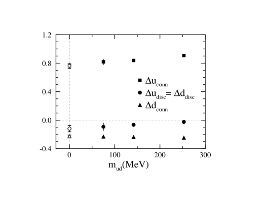
Figure 3: Axial charges for $u$ and $d$ quarks as a function of degenerate $u$ and $d$ quark mass. Open symbols denote the values extrapolated linearly to the chiral limit.

Table 2: Proton axial charges in the $\overline{\rm MS}$ scheme as a function of $K_{ud}$. $\Delta d_{\rm disc}$ equals $\Delta u_{\rm disc}$. Values at $K_{c}$ are obtained by a linear fit in $1/K$.

$K_{ud}$	$\Delta u_{\rm conn}$	$\Delta d_{\rm conn}$	$\Delta u_{\rm disc}$	$\Delta s_{\rm disc}$
				$K_{s}$=0.1665	0.1640	0.1600
0.1600	$0.9071(92)$	$-0.2470(35)$	$-0.025(10)$	$-0.025(10)$	$-0.035(12)$	$-0.042(15)$
0.1640	$0.839(19)$	$-0.2382(87)$	$-0.066(23)$	$-0.049(19)$	$-0.066(23)$	$-0.076(27)$
0.1665	$0.818(39)$	$-0.231(23)$	$-0.093(54)$	$-0.068(35)$	$-0.084(46)$	$-0.093(54)$
$K_{c}$	$0.763(35)$	$-0.226(17)$	$-0.119(44)$

We present the axial charges for $u$, $d$ and $s$ quarks in Fig. 3 as a function of the bare quark mass $m_{ud}$ in physical units. As we already remarked the values of the disconnected contribution(circles) are small and negative. Their magnitude increases slightly toward the chiral limit, while the connected contributions decrease.

We calculate the physical values of matrix elements in the following way. For $u$ and $d$ quarks, we estimate the sum of disconnected and connected contributions by first combining the two contributions in the ratio $R_{A_{q}}(t)$ and then fitting the result to the linear form (2) over $5\leq t\leq 10$ for each $K_{ud}$. The fitted values are extrapolated linearly to the chiral limit $m_{ud}=0$, where we neglect the degenerate $u$ and $d$ quark mass (see Table 1). For the strange quark contribution similar extrapolations to $m_{ud}=0$ are made for each $K_{s}$, and their results in turn are interpolated to the strange quark mass $m_{s}$. This analysis yields for the quark contribution to proton spin,

$$\Delta\Sigma=\Delta u+\Delta d+\Delta s=+0.638(54)-0.347(46)-0.109(30)=+0.18(10).$$ (19)

These values, notably the sign and magnitude of the strange quark contribution, show a reasonable agreement with the phenomenological estimate $\Delta\Sigma=0.10^{+0.17}_{-0.11}$[13].

Possible sources of systematic errors in our results are scaling violation effects due to a fairly large lattice spacing $a\approx 0.14$fm at $\beta=5.7$, quenched approximation and uncertainties in the perturbative estimate of the renormalization factor (18). For the first two systematic errors we can roughly estimate its magnitude from our result of the flavor non-singlet axial charge $g_{A}=\Delta u-\Delta d=0.985(25)$ at $m_{ud}=0$, which is about $25\%$ smaller than the experimental value $g_{A}=1.2601(25)$[22]. The small value of $g_{A}$, possibly arising from these uncertainties, suggest that our result for $\Delta\Sigma$ might be underestimating the continuum value by a similar magnitude. For the perturbative renormalization factor we note that the lack of two-loop calculation for the flavor singlet lattice-to-continuum renormalization factor makes it difficult to specify the scale at which $\Delta\Sigma$ is evaluated, although we expect the scale dependence to be weak, being a two-loop effect. These points should be examined in future studies.

5.2 Tensor charges

So far, there exist several model calculations of the tensor charge. Non-relativistic quark model predicts $\delta u=\Delta u=4/3$ and $\delta d=\Delta d=-1/3$, while relativistic quark wave functions with non-vanishing lower components lead to $\delta u=1.17$ and $\delta d=-0.29$ together with the inequality $|\delta q|>|\Delta q|$ $(q=u,d)$[23]. There also exist attempts to calculate $\delta q$ using QCD sum rules $(\delta u=1.33(53),\delta d=0.04(2))$[23, 24] and a chiral quark model $(\delta u=1.12,\delta d=-0.42,\delta s=-0.008)$[25]. The main deficiencies of these model calculations are as follows.

i) the renormalization scale where the matrix elements are evaluated is not clear. The tensor current has an anomalous dimension at the one-loop level, while that of the flavor singlet axial current starts from the two-loop level.

ii) it is hard to estimate the contribution of OZI violating process, especially strange quark contributions, in a reliable manner.

Lattice QCD calculation is free from these problems even in the quenched approximation.

Figure 4: Same as Fig. 3 for $R_{T_{q}}(t)$. Solid lines are linear fits over $6\leq t\leq 11$.

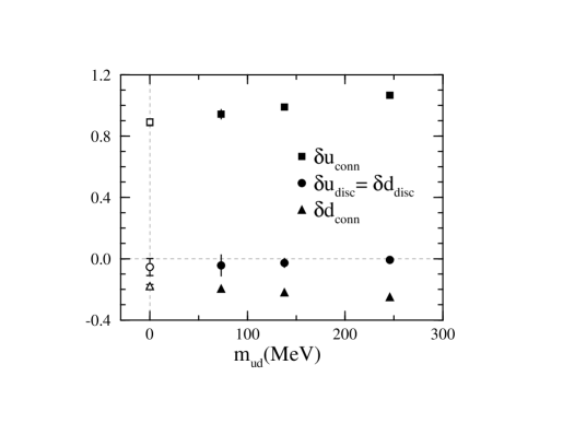
Figure 5: Same as Fig. 3 for the tensor charge.

We calculate the ratio of (2) for the tensor operator $T_{q}={\bar{q}}\sigma_{\mu\nu}q$ $(q=u,d,s)$. The ratio $R_{T_{q}}(t)$ are plotted in Fig. 5 for the case of $K_{ud}=0.164$. Fig. 5(a) shows a clear linear behavior for the connected contributions up to $t\sim 13$, beyond which errors grow rapidly. For the disconnected contribution in Fig. 5(b) the data stay around zero with $100\%$ errors and does not show clear signal of a linear dependence on $t$. We extract the tensor charge both for the connected and disconnected contributions fitting the data of $R_{T_{q}}(t)$ with a linear form (2) over $6\leq t\leq 11$.

The results for $\delta q$ are corrected by the one-loop renormalization factor[17, 21]

$$Z_{T_{q}}(\mu a,\alpha_{\overline{\rm MS}}(1/a))=\left(1-{3K_{q}\over 4K_{c}}\right)\left[1-\left({2\over 3\pi}\ln(\mu a)+0.44\right)\ \alpha_{\overline{\rm MS}}(1/a)\right].$$ (20)

The tensor charges $\delta u$, $\delta d$ and $\delta s$ in the ${\overline{\rm MS}}$ scheme are tabulated in Table 3.

In Fig. 5 we plot the tensor charges as a function of the lattice bare quark mass $m_{ud}$. The connected contributions for $u$ and $d$ quarks decreases in magnitude as the quark mass decreases. This trend is the same as for the axial charge. For the disconnected contribution our result is consistent with zero, which indicates that the OZI violating effects are negligible for the tensor charge.

Table 3: Proton tensor charges at $\mu=1/a$ in the $\overline{\rm MS}$ scheme as a function of $K_{ud}$. $\delta d_{\rm disc}$ equals $\delta u_{\rm disc}$. Values at $K_{c}$ are obtained by a linear fit in $1/K$.

$K_{ud}$	$\delta u_{\rm conn}$	$\delta d_{\rm conn}$	$\delta u_{\rm disc}$	$\delta s_{\rm disc}$
				$K_{s}$=0.1665	0.1640	0.1600
0.1600	1.072(50)	$-0.251(21)$	$-0.008(12)$	$-0.022(16)$	$-0.013(14)$	$-0.008(12)$
0.1640	0.994(11)	$-0.220(52)$	$-0.027(28)$	$-0.041(33)$	$-0.027(28)$	$-0.013(25)$
0.1665	0.948(31)	$-0.196(15)$	$-0.044(69)$	$-0.044(69)$	$-0.035(58)$	$-0.009(51)$
$K_{c}$	0.893(22)	$-0.180(10)$	$-0.054(54)$

To extract the physical tensor charge for $u$ and $d$ quarks the fitted values are linearly extrapolated to the chiral limit $m_{ud}=0$. For the strange quark contribution we first make linear interpolation to the physical strange quark mass $m_{s}a$ at each fixed value of $K_{ud}$ for nucleon, and then the results are linearly extrapolated to the chiral limit. The final results for the tensor charge is

$$\delta\Sigma=\delta u+\delta d+\delta s=+0.839(60)-0.231(55)-0.046(34)=+0.562(88),$$ (21)

where the error of of the sum of $u$, $d$, $s$ contributions are estimated by quadrature.

Due to the smallness of the disconnected contributions, the flavor singlet tensor charge $\delta\Sigma$ is not much suppressed from its quark model value. This is in contrast to the flavor singlet axial charge $\Delta\Sigma$ which suffers from large suppression. The ratio $|\delta q/\Delta q|$ extrapolated to the chiral limit gives $|\delta u/\Delta u|=1.32(15)$ and $|\delta d/\Delta d|=0.67(18)$, which are quantitative different from the prediction of the nonrelativistic quark model $|\delta q/\Delta q|=1$ $(q=u,d)$ and also have qualitative difference from the prediction of relativistic quark models $|\delta q/\Delta q|>1$ $(q=u,d)$ mentioned before. The smallness of $\delta q_{\rm disc}$ could be related to the C (charge conjugation)-odd and chiral-odd nature of the tensor operator $\bar{q}\sigma_{\mu\nu}\gamma_{5}q$ [26].

Possible systematic errors originates from the scaling violation effects and the quenched approximation. We may estimate that the magnitude of these systematic errors is $\sim 20\%$ as for the axial charges. Toward a definitive determination of the tensor charge a repetition of the calculation including dynamical quark effects with smaller lattice spacing is required, which we leave for future investigations.

References

- [1]
- [2] R. L. Jaffe and X. Ji, Nucl. Phys. B375 (1992) 527 and references therein.
- [3] K. Imai, these proceedings
- [4] European Muon Collaboration, J. Ashman et al., Nucl. Phys. B328 (1989) 1.
- [5] Spin Muon Collaboration, D. Adams et al., Phys. Lett. B329 (1994) 399.
- [6] E143 Collaboration, K. Abe et al., Phys. Rev. Lett. 74 (1995) 346.
- [7] E143 Collaboration, K. Abe et al., Phys. Lett. B364 (1995) 61.
- [8] Spin Muon Collaboration, D. Adams et al., Phys. Lett. B357 (1995) 248.
- [9] E143 Collaboration, K. Abe et al., Phys. Rev. Lett. 75 (1995) 25.
- [10] Spin Muon Collaboration, D. Adams et al., hep-ex/9702005.
- [11] E142 Collaboration, P. L. Anthony et al., Phys. Rev. D54 (1996) 6620.
- [12] E154 Collaboration, K. Abe et al., Phys. Rev. Lett. 79 (1997) 26.
- [13] G. Altarelli, R. D. Ball, S. Forte and G. Ridolfi, Nucl. Phys. B496 (1997) 337.
- [14] M. Fukugita, Y. Kuramashi, M. Okawa and A. Ukawa, Phys. Rev. Lett. 75 (1995) 2092.
- [15] S. Aoki, M. Doui, T. Hatsuda and Y. Kuramashi, Phys. Rev. D56 (1997) 433.
- [16] M. Okawa, Nucl. Phys. B (Proc. Suppl.) 47 (1996) 160.
- [17] G. Martinelli and Y.-C. Zhang, Phys. Lett. B123 (1983) 433.
- [18] C. Bernard et al., in Lattice Gauge Theory: A Challenge in Large-Scale Computing, eds. B. Bunk et al. (Plenum, New York, 1986); G. W. Kilcup et al., Phys. Lett. 164B (1985) 347.
- [19] Y. Kuramashi, M. Fukugita, H. Mino, M. Okawa and A. Ukawa, Phys. Rev. Lett. 71 (1993) 2387; Phys. Rev. Lett. 72 (1994) 3448.
- [20] A. X. El-Khadra et al., Phys. Rev. Lett. 69 (1992) 729.
- [21] G. P. Lepage and P. B. Mackenzie, Phys. Rev. D48 (1993) 2250.
- [22] Particle Data Group, Phys. Rev. D54 (1996) 1.
- [23] H. He and X. Ji, Phys. Rev. D52 (1995) 2960; ibid. D54 (1996) 6897.
- [24] B. L. Ioffe and A. Khodjamiraian, Phys. Rev. D51 (1995) 3373.
- [25] H.-C. Kim, M. Polyakov and K. Goeke, Phys. Lett. B387 (1996) 577.
- [26] X. Ji and J. Tang, Phys. Lett. B362 (1995) 182.