The Kaon $B$-parameter with the Wilson Quark Action using Chiral Ward Identities

Abstract

We present a detailed description of the method and results of our calculation of the kaon $B$ parameter using the Wilson quark action in quenched QCD at $\beta=5.9-6.5$. The mixing problem of the $\Delta s=2$ four-quark operators is solved non-perturbatively with full use of chiral Ward identities. We find $B_{K}({\rm NDR},2{\rm GeV})=0.562(64)$ in the continuum limit, which agrees with the value obtained with the Kogut-Susskind quark action.

1 Introduction

The Wilson quark action explicitly breaks chiral symmetry at finite lattice spacing, which causes problems in a number of subjects treated by numerical simulations of lattice QCD. For the calculation of the kaon $B$ parameter $B_{K}$, the problem appears as a non-trivial mixing of the weak $\Delta s=2$ four-quark operator of purely left handed chirality with those of mixed left-right chirality. It has been well known that perturbation theory does not work effectively for solving this mixing problem[1], and most calculations of $B_{K}$ have tried to resolve the mixing non-perturbatively with the aid of chiral perturbation theory[2]. This method, however, has not been successful, since it contains large systematic uncertainties from higher order effects of chiral perturbation theory which survive even in the continuum limit.

An essential step for a precise determination of $B_{K}$ is to control the operator mixing non-perturbatively without resort to any effective theories. The failure of the perturbative approach suggests that higher order corrections in terms of the coupling constant might be large in the mixing coefficients. Presence of large $O(a)$ corrections in the coefficients is also a possibility. In order to deal with this problem, the Rome group has proposed the method of non-perturbative renormalization(NPR)[3], which shows an improvement of the chiral behavior for the $\Delta s=2$ operator[4]. Recently we have proposed an alternative non-perturbative method to solve the operator mixing problem which is based on the use of chiral Ward identities[5]. This method fully incorporates the chiral properties of the Wilson action. Our numerical results show that the renormalized $\Delta s=2$ operator constructed with this method has good chiral behavior with the mixing coefficients having small momentum scale dependence.

The chief findings of our calculation have already been presented in Ref. [5]. In this report we give a detailed description of the implementation of our method and the results of our analyses.

2 Formulation of the method

Let us consider flavor $SU(3)$ chiral variation defined by

$$\delta^{a}\psi(x) = i\frac{\lambda^{a}}{2}\gamma_{5}\psi(x),$$ (1)

$$\delta^{a}{\bar{\psi}}(x) = {\bar{\psi}}(x)i\frac{\lambda^{a}}{2}\gamma_{5},$$ (2)

where $\lambda^{a}$ $(a=1,\cdots,8)$ are the flavor matrices normalized as Tr$(\lambda^{a}\lambda^{b})=2\delta^{ab}$. We consider a set of weak operators in the continuum $\{\hat{O}_{i}\}$ which closes under flavor chiral rotations $\delta^{a}\hat{O}_{i}=ic^{a}_{ij}\hat{O}_{j}$. These operators are given by linear combinations of a set of lattice local operators $\{O_{\alpha}\}$ as $\hat{O}_{i}=\sum_{\alpha}Z_{i\alpha}O_{\alpha}$.

We choose the mixing coefficients $Z_{i\alpha}$ such that the Green functions of $\{\hat{O}_{i}\}$ with quarks in the external states satisfy the chiral Ward identity to $O(a)$. This identity can be derived in a standard manner[6] and takes the form given by

$$-2\rho Z_{A}^{\rm ext}\langle\sum_{x}P^{a}(x)\hat{O}_{i}(0)\prod_{k}\tilde{\psi}(p_{k})\rangle$$

$$+c^{a}_{ij}\langle\hat{O}_{j}(0)\prod_{k}\tilde{\psi}(p_{k})\rangle$$ (3)

$$-i\sum_{l}\langle\hat{O}_{i}(0)\prod_{k\neq l}\tilde{\psi}(p_{k})\delta^{a}\tilde{\psi}(p_{l})\rangle+O(a)=0,$$

where $p_{k}$ is the momentum of the external quark, $Z_{A}^{\rm ext}$ and $\rho=(m-\delta m)/Z_{A}^{\rm ext}$ are constants to be determined from the Ward identities for the axial vector currents[7], and $P^{a}$ is the pseudoscalar density of flavor $a$ defined by $P^{a}(x)={\bar{\psi(x)}}\frac{1}{2}\lambda^{a}\gamma_{5}{\psi(x)}$. We note that the first term in (3) comes from the chiral variation of the Wilson quark action and the third represents the chiral rotation of the external fields.

The four-quark operator relevant for $B_{K}$ is given by $\hat{O}_{VV+AA}=(\bar{s}\gamma_{\mu}d)(\bar{s}\gamma_{\mu}d)+(\bar{s}\gamma_{\mu}\gamma_{5}d)(\bar{s}\gamma_{\mu}\gamma_{5}d)$ where $()$ means color trace. To fix the mixing coefficients for the lattice four-quark operators, we may choose a particular $SU(3)$ flavor chiral rotation to be applied for $\hat{O}_{VV+AA}$. Avoiding flavor rotations that yield operators which have Penguin contractions and hence mix with lower dimension operators, we employ the $\lambda^{3}={\rm diag}(1,-1,0)$ chiral rotation, under which $\hat{O}_{VV+AA}$ and $\hat{O}_{VA}=(\bar{s}\gamma_{\mu}d)(\bar{s}\gamma_{\mu}\gamma_{5}d)$ form a minimal closed set of the operators.

Since $\hat{O}_{VV+AA}$ and $\hat{O}_{VA}$ are dimension six operators with $\Delta s=2$, we can restrict ourselves to dimension six operators for the construction of the lattice operators corresponding to them. The set of lattice bare operators with even parity is given by

$$\begin{array}[]{lll}VV&=&(\bar{s}\gamma_{\mu}d)(\bar{s}\gamma_{\mu}d)\\ AA&=&(\bar{s}\gamma_{\mu}\gamma_{5}d)(\bar{s}\gamma_{\mu}\gamma_{5}d)\\ SS&=&(\bar{s}d)(\bar{s}d)\\ PP&=&(\bar{s}\gamma_{5}d)(\bar{s}\gamma_{5}d)\\ TT&=&(\bar{s}\sigma_{\mu\nu}d)(\bar{s}\sigma_{\mu\nu}d)/2\\ \end{array}$$ (4)

and the set with odd parity is

$$\begin{array}[]{lll}VA&=&(\bar{s}\gamma_{\mu}d)(\bar{s}\gamma_{\mu}\gamma_{5}d)\\ SP&=&(\bar{s}d)(\bar{s}\gamma_{5}d)\\ T{\tilde{T}}&=&(\bar{s}\sigma_{\mu\nu}d)(\bar{s}\sigma_{\mu\nu}\gamma_{5}d)/2\\ \end{array}$$ (5)

where $\sigma_{\mu\nu}=[\gamma_{\mu},\gamma_{\nu}]/2$. In terms of these operators we construct the Fierz eigenbasis, which we find convenient when taking fermion contractions for evaluating the Green functions in (3),

$$\begin{array}[]{ll}O_{0}=\left(VV+AA\right)/2&(+,+)\\ O_{1}=\left(SS+TT+PP\right)/2&(+,+)\\ O_{2}=\left(SS-TT/3+PP\right)/2&(-,+)\\ O_{3}=\left(VV-AA\right)/2+\left(SS-PP\right)&(-,+)\\ O_{4}=\left(VV-AA\right)/2-\left(SS-PP\right)&(+,+)\\ \end{array}$$ (6)

$$\begin{array}[]{ll}O_{5}=VA&(+,+)\\ O_{6}=SP+T{\tilde{T}}/2&(+,-)\\ O_{7}=SP-T{\tilde{T}}/6&(-,-)\\ \end{array}$$ (7)

Here the first sign after each equation denotes the Fierz eigen value and the second the $CPS$[1] eigen value. We note that the Fierz eigen basis we employ is different from the basis chosen by the Rome group[4] based on one-loop perturbation theory.

The parity odd operators $O_{6,7}$ are $CPS$ odd while $O_{5}$ is $CPS$ even, and hence $O_{5}$ does not mix with $O_{6,7}$ under renormalization. Therefore the mixing structure of these operators is given by

$$\frac{\hat{O}_{VV+AA}}{2Z_{VV+AA}}=O_{0}+z_{1}O_{1}+\cdots+z_{4}O_{4},$$ (8)

$$\frac{\hat{O}_{VA}}{Z_{VA}}=z_{5}O_{5},$$ (9)

where $Z_{VV+AA}$ and $Z_{VA}$ are overall renormalization factors.

Let us consider an external state consisting of two $s$ quarks and two $d$ quarks, all having an equal momentum $p$. Under $\lambda^{3}$ chiral rotation the Ward identity (3) for such an external state takes the following form:

$$\begin{array}[]{l}F_{VV+AA}\equiv\\ -2\rho Z_{A}^{\rm ext}\langle\sum_{x}P^{a}(x)\frac{1}{2}{\hat{O}}_{VV+AA}(0)({\tilde{s}}{\tilde{s}}{\tilde{\bar{d}}}{\tilde{\bar{d}}})(p)\rangle\\ -\langle\hat{O}_{VA}(0)({\tilde{s}}{\tilde{s}}{\tilde{\bar{d}}}{\tilde{\bar{d}}})(p)\rangle\\ -\langle\frac{1}{2}{\hat{O}}_{VV+AA}(0)\delta^{3}({\tilde{s}}{\tilde{s}}{\tilde{\bar{d}}}{\tilde{\bar{d}}})(p)\rangle+O(a)=0,\end{array}$$ (10)

$$\begin{array}[]{l}F_{VA}\equiv\\ -2\rho Z_{A}^{\rm ext}\langle\sum_{x}P^{a}(x){\hat{O}}_{VA}(0)({\tilde{s}}{\tilde{s}}{\tilde{\bar{d}}}{\tilde{\bar{d}}})(p)\rangle\\ -\langle\frac{1}{2}{\hat{O}}_{VV+AA}(0)({\tilde{s}}{\tilde{s}}{\tilde{\bar{d}}}{\tilde{\bar{d}}})(p)\rangle\\ -\langle{\hat{O}}_{VA}(0)\delta^{3}({\tilde{s}}{\tilde{s}}{\tilde{\bar{d}}}{\tilde{\bar{d}}})(p)\rangle+O(a)=0,\end{array}$$ (11)

where $({\tilde{s}}{\tilde{s}}{\tilde{\bar{d}}}{\tilde{\bar{d}}})(p)$ and $\delta^{3}({\tilde{s}}{\tilde{s}}{\tilde{\bar{d}}}{\tilde{\bar{d}}})(p)$ represent ${\tilde{s}}(p){\tilde{s}}(p){\tilde{\bar{d}}}(p){\tilde{\bar{d}}}(p)$ and ${\tilde{s}}(p){\tilde{s}}(p)({\tilde{\bar{d}}}(p)\gamma_{5}/2){\tilde{\bar{d}}}(p)$ $+{\tilde{s}}(p){\tilde{s}}(p){\tilde{\bar{d}}}(p)({\tilde{\bar{d}}}(p)\gamma_{5}/2)$, respectively. We obtain the amputated Green functions for $F_{VV+AA}$ and $F_{VA}$ by truncating the external quark propagators according to

$$\begin{array}[]{l}\Gamma_{VV+AA,VA}\equiv\\ G_{s}^{-1}(p)G_{s}^{-1}(p)F_{VV+AA,VA}G_{\bar{d}}^{-1}(p)G_{\bar{d}}^{-1}(p),\end{array}$$ (12)

where $G_{q}^{-1}$ denotes the inverse quark propagator with the flavor $q$.

Let $P_{i}$ $(i=0,\cdots,7)$ be the projection operator corresponding to the four-quark operators in the Fierz eigenbasis $O_{i}$ $(i=0,\cdots,7)$. For example, we have

$$P_{0}^{\alpha\beta\delta\lambda}=\frac{1}{64}\left[\gamma_{\mu}^{\alpha\beta}\gamma_{\mu}^{\delta\lambda}+(\gamma_{\mu}\gamma_{5})^{\alpha\beta}(\gamma_{\mu}\gamma_{5})^{\delta\lambda}\right].$$ (13)

Since QCD conserves parity one can write

$$\Gamma_{VV+AA}/Z_{VV+AA}=\Gamma_{5}P_{5},$$ (14)

$$\Gamma_{VA}/Z_{VA}=\Gamma_{0}P_{0}+\Gamma_{1}P_{1}+\cdots+\Gamma_{4}P_{4}.$$ (15)

Expressing ${\hat{O}_{VV+AA,VA}}$ in (3) in terms of lattice operators, we obtain six equations for the five coefficients $z_{1},\cdots,z_{5}$:

$$\Gamma_{i}=c^{i}_{0}+c^{i}_{1}z_{1}+\cdots+c^{i}_{5}z_{5}=O(a),\,i=0,\cdots,5\,$$ (16)

This gives an overconstrained set of equations, and we may choose any five equations to exactly vanish to solve for $z_{i}$: the remaining equation should automatically be satisfied to $O(a)$. We choose four equations to be those for $i=1,\cdots,4$, since $O_{1},\cdots,O_{4}$ do not appear in the continuum. The choice of the fifth equation, $i=0$ or 5, is more arbitrary. We have checked that either $\Gamma_{0}=0$ or $\Gamma_{5}=0$ leads to a consistent result to $O(a)$ for $z_{1},\cdots,z_{4}$ in the region $pa\hbox to0.0pt{\lower 3.5pt\hbox{$\mathchar 0\relax\sim$}\hss}\raise 1.0pt\hbox{$<$}1$. In the present analysis we choose $\Gamma_{5}=0$.

Table 1: Parameters of our simulations. See text for details.

$\beta$	5.9	6.1	6.3	6.5
$L^{3}\times T$	$24^{3}\times 64$	$32^{3}\times 64$	$40^{3}\times 96$	$48^{3}\times 96$
#conf.	300	100	50	24
skip	2000	2000	5000	8000
$K$	0.15862	0.15428	0.15131	0.14925
	0.15785	0.15381	0.15098	0.14901
	0.15708	0.15333	0.15066	0.14877
	0.15632	0.15287	0.15034	0.14853
fitting range ($m_{\pi},m_{\rho}$)	$13-21$	$15-25$	$18-28$	$21-31$
fitting range ($B_{K}$)	$19-46$	$25-40$	$33-64$	$36-61$
$K_{c}$	$0.15986(3)$	$0.15502(2)$	$0.15182(2)$	$0.14946(3)$
$a^{-1}$(GeV)	1.95(5)	2.65(11)	3.41(20)	4.30(29)
$La$(fm)	2.4	2.4	2.3	2.2
$\alpha_{\overline{\rm MS}}(1/a)$	0.1922	0.1739	0.1596	0.1480
$m_{s}a/2=m_{d}a/2$	$0.0294(14)$	$0.0198(16)$	$0.0144(17)$	$0.0107(16)$
$\delta_{p^{2}}$	$1.11$	$1.11$	$1.15$	$1.12$
${p^{*}}^{2}a^{2}$	$0.9595$	$0.5012$	$0.2988$	$0.2056$

The overall factor $Z_{VV+AA}$ is determined by the NPR method[3]. We calculate the amputated Green function,

$$\begin{array}[]{l}G_{s}^{-1}(p)G_{s}^{-1}(p)\langle\frac{1}{2}{\hat{O}}_{VV+AA}(0)({\tilde{s}}{\tilde{s}}{\tilde{\bar{d}}}{\tilde{\bar{d}}})(p)\rangle\\ \times G_{\bar{d}}^{-1}(p)G_{\bar{d}}^{-1}(p)={\hat{\Gamma}}_{VV+AA}(p)P_{0}+\cdots,\end{array}$$ (17)

and impose the following condition,

$$Z_{VV+AA}(p)Z_{q}^{-2}(p){\hat{\Gamma}}_{VV+AA}(p)=1,$$ (18)

where $Z_{q}(p)$ is the quark wave-function renormalization factor which is calculated from

$$Z_{q}(p)=\frac{{\rm Tr}\left(-i\sum_{\mu}\gamma_{\mu}{\rm sin}(p_{\mu})G_{q}^{-1}(p)\right)}{4\sum_{\mu}{\rm sin}^{2}(p_{\mu})}.$$ (19)

We convert the matrix elements on the lattice into those of the $\overline{\rm MS}$ scheme in the continuum with naive dimensional regularization (NDR) and renormalized at the scale $\mu=2$GeV[8]:

$$B_{K}({\rm NDR},\mu)=B_{K}(p,1/a)$$ (20)

$$\times\left[1+\frac{\alpha_{s}(\mu)}{4\pi}\left(-4\,{\rm log}\left(\frac{\mu}{p}\right)-\frac{14}{3}+8\log 2\right)\right],$$

where

$$B_{K}(p,1/a)=\frac{\langle{\bar{K}}^{0}|\hat{O}_{VV+AA}|K^{0}\rangle}{\frac{8}{3}|\langle 0|{\hat{A}}|K^{0}\rangle|^{2}}$$ (21)

with $p$ the momentum at which the mixing coefficients are evaluated. The axial vector current in the denominator is given by ${\hat{A}}=Z_{A}\bar{s}\gamma_{4}\gamma_{5}d$ with $Z_{A}$ the renormalization factor determined by the NPR method.

For comparative purpose we also calculate $B_{K}$ with perturbative mixing coefficients, for which we use the one-loop expression in Ref. [9] after applying a finite correction in conversion to the NDR scheme together with the tadpole improvement with $\alpha_{\overline{\rm MS}}(1/a)$.

Let us remark here that the equations obtained in the NPR method [4] corresponds to $\Gamma_{i}=0$ for $i=1,\cdots,4$ in which the contributions of the first and the third term in the Ward identity (3) are dropped. In particular the NPR method neglects the quark mass contributions coming from the first term of (3). As may be expected from this, the NPR method is equivalent to the Ward identities in the limit of large external virtualities[3, 4].

3 Parameters of numerical simulation

Our calculations are made with the Wilson quark action and the plaquette action at $\beta=5.9-6.5$ in quenched QCD. Table 1 summarizes our run parameters. Gauge configurations are generated with the 5-hit pseudo heat-bath algorithm. At each value of $\beta$ four values of the hopping parameter $K$ are adopted such that the physical point for the $K$ meson can be interpolated. The critical hopping parameter $K_{c}$ is determined by extrapolating results for $m_{\pi}^{2}$ for the four hopping parameters linearly in $1/2K$ to $m_{\pi}^{2}=0$. We take the down and strange quarks to be degenerate. The value of half the strange quark mass $m_{s}a/2$ is then estimated from $m_{K}/m_{\rho}=0.648$.

The physical size of lattice is chosen to be approximately constant at $La\approx 2.4$fm where the lattice spacing is determined from $m_{\rho}=770$MeV. To calculate the perturbative renormalization factors, we employ the strong coupling constant at the scale $1/a$ in the $\overline{\rm MS}$ scheme, evaluated by a two-loop renormalization group running starting from $g^{2}_{\overline{\rm MS}}(\pi/a)=P_{\rm av}/g^{2}_{latt}+0.0246$ with $P_{\rm av}$ the averaged value of the plaquette.

The renormalization factors $Z_{VV+AA}$, $Z_{A}$ and the mixing coefficients $z_{i}$ $(i=1,\cdots,5)$ are calculated for a set of external quark momenta $p^{(i)}$ $(i=1,\cdots,\sim 40)$, which is chosen recursively according to the condition that the $(i+1)$-th momentum $p^{(i+1)}a$ is the minimum number satisfying ${p^{(i+1)}}^{2}a^{2}\geq\delta_{p^{2}}\cdot{p^{(i)}}^{2}a^{2}$ with $p^{(1)}a=2\pi/T$ where $T$ denotes the temporal lattice size. We employ $p^{*}\approx 2$GeV among $p^{(i)}$ for the analysis of $B_{K}$. Errors are estimated by the single elimination jackknife method for all measured quantities throughout this work.

4 Calculational procedure

Our calculations are carried out in two steps. We first calculate $Z_{VV+AA}$, $Z_{A}$ and $z_{i}$ using the quark Green functions having finite space-time momenta. For this purpose quark propagators are solved in the Landau gauge for the point source located at the origin with the periodic boundary condition imposed in all four directions. For calculating the first term of the Ward identity (3), we use the source method[10] to insert the pseudoscalar density. The point source quark propagators are also used for calculating $\pi$ and $\rho$ propagators and to extract their masses from them.

The $B_{K}$ parameter is extracted from the ratio

$$R(t^{\prime}) = \frac{\langle O_{{\bar{K}}^{0}}(T){\hat{O}}_{VV+AA}(t^{\prime})O_{K^{0}}^{\dagger}(1)\rangle}{\frac{8}{3}\langle O_{{\bar{K}}^{0}}(T){\hat{A}}(t^{\prime})\rangle\langle{\hat{A}}(t^{\prime})O_{K^{0}}^{\dagger}(1)\rangle}$$

$$\longrightarrow B_{K}(p^{*},1/a)/L^{3}\;\;{\rm for}\;\;1\ll t^{\prime}\ll T,$$

where various operators are defined by $O_{K^{0}}(t)=\sum_{\vec{x}}{\bar{s}}(\vec{x},t)\gamma_{5}d(\vec{x},t)$, $O_{\bar{K}^{0}}(t)$$=$$\sum_{\vec{x}}{\bar{d}}(\vec{x},t)\gamma_{5}s(\vec{x},t)$, ${\hat{O}}_{VV+AA}(t)$$=$$\sum_{i=0}^{4}\sum_{\vec{x}}Z_{VV+AA}z_{i}O_{i}(\vec{x},t)$ and ${\hat{A}}(t)$$=$$\sum_{\vec{x}}Z_{A}{\bar{s}}(\vec{x},t)\gamma_{4}\gamma_{5}d(\vec{x},t)$. The contribution of the operators $O_{i}$ $(i=0,\cdots,4)$ to $B_{K}(p^{*},1/a)$ can be obtained similarly from

$$R^{i}(t^{\prime})=\frac{\langle O_{{\bar{K}}^{0}}(T){\hat{O}}_{i}(t^{\prime})O_{K^{0}}^{\dagger}(1)\rangle}{\frac{8}{3}\langle O_{{\bar{K}}^{0}}(T){\hat{A}}(t^{\prime})\rangle\langle{\hat{A}}(t^{\prime})O_{K^{0}}^{\dagger}(1)\rangle},$$ (23)

where ${\hat{O}_{i}}(t^{\prime})=\sum_{\vec{x}}Z_{VV+AA}z_{i}O_{i}(\vec{x},t^{\prime})$. For calculation of these ratios we solve quark propagators without gauge fixing employing wall sources placed at the edges of lattice where the Dirichlet boundary condition is imposed in the time direction. We obtain $B_{K}$ at $m_{s}/2$ by quadratically interpolating the data at the four hopping parameters.

5 Results for mixing coefficients

Figure 1: Mixing coefficients $z_{1},\cdots,z_{4}$ plotted as a function of external momentum squared $(pa)^{2}$ for $K=0.15034$ at $\beta=6.3$. Vertical line corresponds to $p^{*}\approx 2$ GeV.

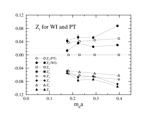
Figure 2: Comparison of the mixing coefficients $z_{1},\cdots,z_{4}$ evaluated at ${p^{*}}\approx 2$ GeV using the Ward identity (WI; solid symbols) and perturbative (PT; open symbols) methods. The coefficients are plotted as a function of $m_{\rho}a$.

Figure 3: Same as Fig. 1 for mixing coefficient $z_{5}$.

Figure 4: Mixing coefficient $z_{5}$ evaluated at ${p^{*}}\approx 2$ GeV using the Ward identity method as a function of $m_{\rho}a$.

In Fig. 1 we plot a typical result for the mixing coefficients $z_{i}$ $(i=1,\cdots,4)$ as a function of the external quark momenta for the case of $K=0.15034$ at $\beta=6.3$. The mixing coefficients shows only weak dependence over a wide momentum range $0.02\hbox to0.0pt{\lower 3.5pt\hbox{$\mathchar 0\relax\sim$}\hss}\raise 1.0pt\hbox{$<$}p^{2}a^{2}\hbox to0.0pt{\lower 3.5pt\hbox{$\mathchar 0\relax\sim$}\hss}\raise 1.0pt\hbox{$<$}1.0$, albeit $z_{1}$ and $z_{2}$ have large errors in the small momentum region $p^{2}a^{2}\hbox to0.0pt{\lower 3.5pt\hbox{$\mathchar 0\relax\sim$}\hss}\raise 1.0pt\hbox{$<$}0.1$. This enables us to evaluate the mixing coefficients with small errors at the scale $p^{*}\approx 2$GeV, which always falls within the range of a plateau for our runs at $\beta=5.9-6.5$.

At the workshop Talevi[11] presented a reanalysis of the results of the Rome group for the mixing coefficients in the Fierz eigen basis, reporting that the momentum dependence in this basis is similar to that of our results in Fig. 1. Their simulations are made at $\beta=6.2$ with the Clover action. For a more detailed comparison, a parallel analysis with the NPR and Ward identity methods employing the same quark action on the same set of configurations would be desirable.

In Fig. 2 we compare the mixing coefficients $z_{i}$ $(i=1,\cdots,4)$ evaluated at the scale $p^{*}$ (filled symbols) with the perturbative values obtained with $\alpha_{\overline{\rm MS}}(1/a)$ (open symbols) as a function of lattice spacing. We observe that the $a$ dependence for the mixing coefficients determined from the Ward identities is steeper compared to that for the perturbative estimates. The magnitude of each mixing coefficient for the Ward identity method varies nearly in proportion to $a$, which reduces by $50\%$ between $m_{\rho}a\approx 0.4$ and $m_{\rho}a\approx 0.2$.

We remark that a large value of $z_{2}$ determined by the Ward identities sharply contrasts with the one-loop perturbative result $z_{2}=0$. For the other coefficients, the perturbative results agree with the non-perturbative ones in sign and rough orders of magnitude. However, they differ in quantitative detail. We find that the magnitudes of $z_{4}$ are larger than those of $z_{3}$ for all values of $\beta$, which is contrary to the perturbative result.

For our study of the $B$ parameter the mixing coefficient $z_{5}$ for the parity odd operator ${\hat{O}_{VA}}$ is not directly relevant. For completeness we plot a typical result in Fig. 3. The data shows a scale dependence which is stronger than those of $z_{i}$ $(i=1,\cdots,4)$ for parity even operators toward large momenta. We do not find this to be particularly alarming since $z_{5}$ evaluated for a fixed physical scale $p^{*}$ approaches unity toward the continuum limit as shown in Fig. 4.

6 Chiral behavior

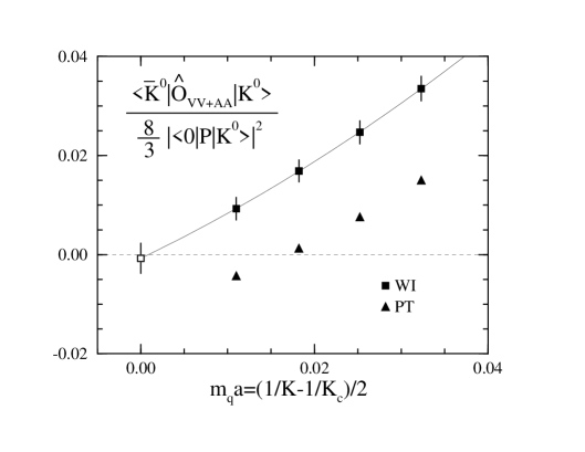
Figure 5: Test of the chiral behavior of $\langle\bar{K}^{0}|\hat{O}_{VV+AA}|K^{0}\rangle/(8/3)/|\langle 0|P|K^{0}\rangle|^{2}$ for the WI and PT methods at $\beta=6.3$. The solid curve is a quadratic extrapolation to the chiral limit.

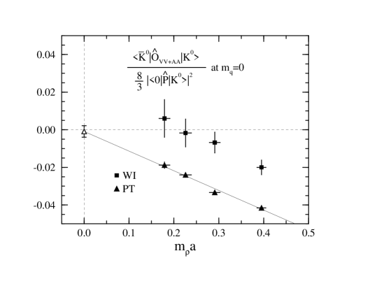
Figure 6: $\langle\bar{K}^{0}|\hat{O}_{VV+AA}|K^{0}\rangle/(8/3)/|\langle 0|\hat{P}|K^{0}\rangle|^{2}$ at $m_{q}=0$ for the WI and PT methods as a function of $a$. The operators are renormalized at 2 GeV in the NDR scheme. For both methods we use the same $\hat{P}$ perturbatively corrected with the tadpole improvement. The solid line is a linear extrapolation to the continuum limit.

Let us examine the chiral property of the operator $\hat{O}_{VV+AA}$. In Fig. 5 we show the chiral behavior of the ratio $\langle{\bar{K}}^{0}|\hat{O}_{VV+AA}|K^{0}\rangle/(8/3)$ $/|\langle 0|P|K^{0}\rangle|^{2}$ at $\beta=6.3$, where WI stands for our method using chiral Ward identities and PT for tadpole-improved one-loop perturbation theory. The solid line represents a quadratic extrapolation of the Ward identity result in the bare quark mass $m_{q}a=(1/K-1/K_{c})/2$. The extrapolated value at $m_{q}=0$ is consistent with zero, demonstrating a significant improvement of the chiral behavior compared to the perturbative result plotted with triangles.

We plot in Fig. 6 the values of the ratio extrapolated to $m_{q}=0$ as a function of lattice spacing, where the pseudoscalar density $\hat{P}$ in the denominator is renormalized perturbatively for both WI and PT cases (numerical results are given in Table 2 below). The ratio for the Ward identity method becomes consistent with zero at the lattice spacing $m_{\rho}a\hbox to0.0pt{\lower 3.5pt\hbox{$\mathchar 0\relax\sim$}\hss}\raise 1.0pt\hbox{$<$}0.3(a\hbox to0.0pt{\lower 3.5pt\hbox{$\mathchar 0\relax\sim$}\hss}\raise 1.0pt\hbox{$<$}0.08$fm).

In the perturbative approach with the one-loop mixing coefficients, chiral breaking effects are expected to appear as terms of $O(g^{4})$ and $O(a)$ for the Wilson quark action. A roughly linear behavior of our results for the perturbative method is consistent with the presence of an $O(a)$ term. Making a linear extrapolation to the continuum limit $a\to 0$, we observe that the chiral behavior is recovered. This may suggest that the $O(g^{4})$ terms in the mixing coefficients left out in the one-loop treatment are actually small.

7 Results for $B_{K}$

Figure 7: Ratio $R(t^{\prime})$ for $K=0.15034$ at $\beta=6.3$. Solid lines denote the fitted result and a one standard deviation error band.

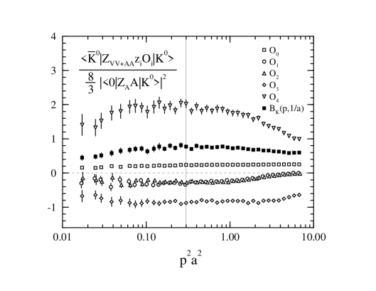
Figure 8: Contribution of the operators $O_{i}$ $(i=0,\cdots,4)$ to $B_{K}(p,1/a)$ with $z_{i}$ determined by the WI method for $K=0.15034$ at $\beta=6.3$. Vertical line corresponds to $p^{*}\approx 2$ GeV.

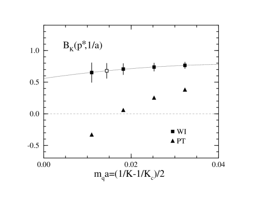
Figure 9: Quark mass dependences of $B_{K}(p^{*},1/a)$ for the WI and PT method at $\beta=6.3$. The open symbol is a quadratical interpolation of the data to $m_{s}/2$.

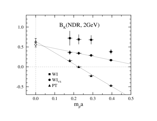
Figure 10: $B_{K}($NDR, 2GeV) plotted as a function of $a$ for the WI, WI_VS and PT methods. The solid lines show linear extrapolations to the continuum limit.

We now turn to the calculation of $B_{K}({\rm NDR},$ $2{\rm GeV})$. In Fig. 7 we present the ratio $R(t^{\prime})$ defined in (4) using the mixing coefficients determined from the Ward identities for $K=0.15034$ at $\beta=6.3$. A good plateau is observed in the range $20\hbox to0.0pt{\lower 3.5pt\hbox{$\mathchar 0\relax\sim$}\hss}\raise 1.0pt\hbox{$<$}t^{\prime}\hbox to0.0pt{\lower 3.5pt\hbox{$\mathchar 0\relax\sim$}\hss}\raise 1.0pt\hbox{$<$}70$. We make a global fit of the ratio $R(t^{\prime})$ to a constant over $33\leq t^{\prime}\leq 64$ for this data set. The three horizontal lines denote the central value of the fit and a one standard deviation error band. We note that the error of the fitted result is roughly equal in magnitude to those of the ratio over the fitted range, while we would usually expect a smaller error for the fitted result. This is because the error of the ratio $R(t^{\prime})$ is governed by those of the mixing coefficients $z_{i}$ $(i=1,\cdots,4)$.

In Fig. 8 a representative result for the contribution of each operator $O_{i}$ $(i=0,\cdots,4)$ to $B_{K}(p,1/a)$ is plotted as a function of the external quark momenta, which is obtained by fitting the ratio $R^{i}(t^{\prime})$ $(i=0,\cdots,4)$ of (23) with a constant over the same fitting range as for $R(t^{\prime})$. The contributions are nearly independent of the external quark momentum in the range $0.05\hbox to0.0pt{\lower 3.5pt\hbox{$\mathchar 0\relax\sim$}\hss}\raise 1.0pt\hbox{$<$}p^{2}a^{2}\hbox to0.0pt{\lower 3.5pt\hbox{$\mathchar 0\relax\sim$}\hss}\raise 1.0pt\hbox{$<$}1.0$ as is expected from the weak scale dependence of the mixing coefficients $z_{i}$ shown in Fig. 1. A decrease in magnitude of the contributions in the small momentum region $p^{2}a^{2}\hbox to0.0pt{\lower 3.5pt\hbox{$\mathchar 0\relax\sim$}\hss}\raise 1.0pt\hbox{$<$}0.05$ originates from the scale dependence of the overall renormalization factor $Z_{VV+AA}/Z_{A}^{2}$ estimated non-perturbatively.

An important observation is that the value of $B_{K}(p,1/a)$ is a result of a large cancellation between the amplitudes of $z_{i}O_{i}$ where each amplitude of the mixing operator $z_{i}O_{i}$ $(i=1,\cdots,4)$ is comparable to or larger than that of $O_{0}$. This is the reason why calculations of $B_{K}$ with the Wilson quark action is difficult.

We plot the quark mass dependence of $B_{K}(p^{*},1/a)$ at $\beta=6.3$ in Fig. 9. We observe that the results for the PT method seems to diverge toward the chiral limit, while those for the WI method stays finite. Interpolating the data for the four hopping parameters quadratically to $m_{s}/2$ we obtain the value of $B_{K}(p^{*},1/a)$ at the physical point.

Let us note that the perturbative results have quite small errors compared to those of the Ward identity method. This is because the mixing coefficients are definitely given for the perturbative method. For a precise determination of $B_{K}$ with the Ward identity method it is of great importance to reduce the errors of the mixing coefficients. For this purpose methods have to be devised to effectively compute quark propagators for a large set of momenta with good precision.

Table 2: Results for $B_{K}($NDR, 2GeV) for WI, WI_VS and PT methods as a function of $\beta$. Ratio $\langle{\bar{K}}^{0}|\hat{O}_{VV+AA}|K^{0}\rangle/(8/3)/|\langle 0|{\hat{P}}|K^{0}\rangle|^{2}$ in the chiral limit is also given.

$\beta$		5.9	6.1	6.3	6.5	$a=0$
$B_{K}($NDR, 2GeV)	WI	$+0.38(6)$	$+0.68(11)$	$+0.69(12)$	$+0.72(18)$
	WIVS	$+0.168(20)$	$+0.288(29)$	$+0.342(33)$	$+0.360(52)$	$+0.562(64)$
	PT	$-0.468(14)$	$-0.225(22)$	$-0.000(21)$	$+0.156(40)$	$+0.639(76)$
$\left.\frac{\langle{\bar{K}}^{0}|\hat{O}_{VV+AA}|K^{0}\rangle}{\frac{8}{3}|\langle 0|{\hat{P}}|K^{0}\rangle|^{2}}\right|_{m_{q}=0}$	WI	$-0.0200(39)$	$-0.0068(55)$	$-0.0017(74)$	$+0.006(10)$
	PT	$-0.0415(8)$	$-0.0333(10)$	$-0.0240(12)$	$-0.0188(17)$	$-0.0009(31)$

Our final results for $B_{K}({\rm NDR},2{\rm GeV})$ obtained with (20) are presented in Fig. 10 as a function of lattice spacing. The numerical values are listed in Table 2. The method based on the Ward identity (WI) gives a value convergent from a lattice spacing of $m_{\rho}a\approx 0.3$ ($B_{K}\sim 0.6-0.8$). The large error, however, hinders us from making an extrapolation to the continuum limit. Since the origin of the large error is traced to that of the mixing coefficients, we develop an alternative method, which we refer to as WI_VS, in which the denominator of the ratio for extracting $B_{K}$ is estimated with the vacuum saturation of $\hat{O}_{VV+AA}$ constructed by the WI method:

$$B_{K}^{\rm VS}(p^{*},1/a)=\frac{\langle{\bar{K}}^{0}|\hat{O}_{VV+AA}|K^{0}\rangle}{Z_{A}^{2}\sum_{i=0}^{4}z_{i}\langle{\bar{K}}^{0}|O_{i}|K^{0}\rangle_{\rm VS}}.$$ (24)

In this case the fluctuations in the numerator, mainly due to those of the mixing coefficients $z_{i}$, are largely canceled by those in the denominator, and the resulting error in $B_{K}$ is substantially reduced as apparent in Fig. 10. The cost is that the denominator of $B_{K}^{\rm VS}(p^{*},1/a)$ contains the contributions of the pseudoscalar density $\langle{\bar{K}}^{0}|P|0\rangle\langle 0|P|K^{0}\rangle$ besides those of the axial vector current $\langle{\bar{K}}^{0}|{\hat{A}}|0\rangle\langle 0|{\hat{A}}|K^{0}\rangle$, due to which the correct chiral behavior of the denominator is not respected at a finite lattice spacing. While WI and WI_VS methods give different results at a finite lattice spacing, the discrepancy is expected to vanish in the continuum limit. A linear extrapolation in $a$ of the WI_VS results yields $B_{K}({\rm NDR},2{\rm GeV})=0.562(64)$, which we take as the best value in the present work. This value is consistent with a recent JLQCD result with the Kogut-Susskind action, $B_{K}({\rm NDR},2{\rm GeV})=0.587(7)(17)$[12].

Intriguing in Fig. 10 is that the perturbative calculation (PT), which gives completely “wrong” values at $a\neq 0$, also yields the correct result for $B_{K}$, when extrapolated to the continuum limit $a=0$. This is a long extrapolation from negative to positive, but the linearly extrapolated value $B_{K}$(NDR, 2GeV)=0.639(76) is consistent with those obtained with the WI or WI_VS method. We note that a long extrapolation may bring a large error in the extrapolated value.

Finally we mention possible sources of systematic errors in our results from quenching effects and uncertainties for Gribov copies in the Landau gauge. With the Kogut-Susskind quark action it has been observed that the error due to quenched approximation is small [13]. Whether this is supported by calculations with Wilson action we must defer to future studies. For the Gribov problem we only quote an earlier study[14] which suggests that ambiguities in the choice of the Gribov copies induce only small uncertainties comparable to typical statistical errors in current numerical simulations.

8 Conclusions

Our analysis of $B_{K}$ demonstrates the effectiveness of the method of chiral Ward identities for constructing the $\Delta s=2$ operator with the correct chiral property. We have shown that both Wilson and Kogut-Susskind actions give virtually the identical answer for $B_{K}$ in their continuum limit. We may hope that further improvement of our simulations, especially the reduction of the errors for the mixing coefficients, leads to a precise determination of $B_{K}$ with the Wilson quark action. The application of this method for calculations of $B_{B}$ is straightforward.

References

- [1] See, e.g., C. Bernard and A. Soni, Nucl. Phys. B (Proc. Suppl.) 9 (1989) 155.
- [2] M. B. Gavela et al., Nucl. Phys. B306 (1988) 677; C. Bernard and A. Soni, Nucl. Phys. B (Proc. Suppl.) 42 (1995) 391; R. Gupta et al., Phys. Rev. D55 (1997) 4036.
- [3] G. Martinelli et al., Nucl. Phys. B445 (1995) 81.
- [4] A. Donini et al., Phys. Lett. B360 (1995) 83; M. Crisafulli et al., Phys. Lett. B369 (1996) 325; A. Donini et al., Nucl. Phys. B (Proc. Suppl.) 53 (1997) 883.
- [5] JLQCD Collaboration, S. Aoki et al., hep-lat/9705035.
- [6] M. Bochicchio et al., Nucl. Phys. B262 (1985) 331.
- [7] L. Maiani and G. Martinelli, Phys. Lett. B178 (1986) 265.
- [8] M. Ciuchini et al., Z. Phys. C68 (1995) 239.
- [9] G. Martinelli, Phys. Lett. B141 (1984) 395; C. Bernard et al., Phys. Rev. D36 (1987) 3224.
- [10] C. Bernard, T. Draper, G. Hockney, and A. Soni, in Lattice Gauge Theory: A Challenge in Large-Scale Computing, eds. B. Bunk et al. (Plenum, New York, 1986); G. W. Kilcup et al., Phys. Lett. 164B, 347 (1985).
- [11] M. Talevi, these proceedings.
- [12] JLQCD Collaboration, S. Aoki et al., Nucl. Phys. B (Proc. Suppl.) 53 (1997) 341.
- [13] G. Kilcup et al., Nucl. Phys. B (Proc. Suppl.) 53 (1997) 345.
- [14] M. L. Paciello et al., Phys. Lett. B341 (1994) 187.