Resolving Exceptional Configurations

Abstract

In lattice QCD with Wilson fermions, exceptional configurations arise in the quenched approximation at small quark mass. The origin of these large previously uncontrolled lattice artifacts is identified. A simple well-defined procedure (MQA) is presented which removes the artifacts while preserving the correct continuum limit.

1 Introduction

Quenched lattice QCD studies using Wilson-Dirac fermions have encountered large statistical errors in calculations involving very light quarks. A small subset of the gauge configurations seem to play a dominant role in the final results. These “exceptional configurations” have limited studies to quark masses much larger than the up and down quark masses. The large fluctuations resulting from these exceptional configurations appear to be related to the structure of the small eigenvalues of the Wilson-Dirac operator [1, 2, 3].

As I will explain, exceptional configurations arise from a specific lattice artifact associated with the Wilson-Dirac formulation. This artifact is not removed by using the standard Sheikholeslami-Wohlert(Clover) $O(a)$ “improved” action [4]. However, introducing a modified quenched approximation (MQA), removes the dominant part of this artifact and eliminates the exceptional configurations, thereby greatly reducing the noise associated with light quarks. The detailed studies that form the basis of this report are presented elsewhere [5, 6].

2 Eigenvalue Spectrum and Zero Modes

The fermion propagator in a background gauge field, $A_{\mu}(x)$, may be written in terms of a sum over the eigenvalues of the Dirac operator,

$${\cal D}f_{i}=\gamma*Df_{i}=\lambda_{i}f_{i}$$ (1)

and

$$S(x,y;\{A\})=\sum_{eigenvalues}\frac{f_{i}(x;A)\bar{g}_{i}(y,A)}{(\lambda_{i}+m_{0})}$$ (2)

where $f_{i}(x,A)$ and $\bar{g}_{i}(x,A)$ are the corresponding left and right eigenfunctions. The mass dependence of the propagator is determined by the nature of the eigenvalue spectrum of the Dirac operator. In the continuum, the euclidean Dirac operator is skewhermitian and its eigenvalues are purely imaginary or zero. Hence, the fermion propagators only have singularities when $m_{0}=0$. The behavior of the eigenvalue spectrum near zero determines the nature of dynamical chiral symmetry breaking [7]. The zero eigenvalues, or zero modes, are related to topological fluctuations of the background gauge field by the index theorem associated with the chiral gauge anomaly [8].

The lattice formulation of Wilson-Dirac fermions qualitatively modifies the nature of the eigenvalue spectrum. The Wilson-Dirac operator is usually written as

$${\cal D} \equiv D-rW$$ (3)

$$D_{a\alpha\vec{m},b\beta\vec{n}} = \frac{1}{2}(\gamma_{\mu})_{ab}U_{\alpha\beta}(\vec{m}\mu)\delta_{\vec{n},\vec{m}+\hat{\mu}}$$

$$~{}~{}-\frac{1}{2}(\gamma_{\mu})_{ab}U^{\dagger}_{\alpha\beta}(\vec{n}\mu)\delta_{\vec{n},\vec{m}-\hat{\mu}}$$

$$W_{a\alpha\vec{m},b\beta\vec{n}} = \frac{1}{2}\delta_{ab}(U_{\alpha\beta}(\vec{m}\mu)\delta_{\vec{n},\vec{m}+\hat{\mu}}$$

$$~{}~{}~{}~{}~{}+U^{\dagger}_{\alpha\beta}(\vec{n}\mu)\delta_{\vec{n},\vec{m}-\hat{\mu}})$$

where $U(\vec{n}\mu)$ are the link matrices associated with the lattice gauge fields, and the parameter $r$ is usually taken to be $1$. The Wilson-Dirac operator is neither skewhermitian (unless $r=0$) nor hermitian. The Wilson term explicitly breaks chiral symmetry and lifts the doubling degeneracy of the pure lattice Dirac action. As a result the eigenvalue spectrum of the Wilson-Dirac operator is no longer purely imaginary but fills a region of the complex plane. The discrete symmetries of the Wilson-Dirac operator imply that the eigenvalues appear in complex conjugate pairs, $(\lambda,{\lambda}^{*})$ and obey reflection symmetries, $(\lambda,-\lambda)$. In addition, there can be precisely real, nondegenerate eigenvalues [9].

All the properties expected to be important in QCD in four dimensions are present in QED2 and in two dimensions the full set of eigenvalues and eigenvectors can be computed on moderate size lattices [6, 9, 10]. Unlike in the continuum, the real eigenvalues do not occur at a specific value associated with the zero mass limit. In fact, even in a single configuration, there is no unique definition of the massless limit. This limit can only be defined by an ensemble average. These fluctuations in the positions of real eigenvalues is a direct consequence of chiral symmetry breaking which occurs as an artifact of Wilson-Dirac fermions. Furthermore, this fluctuation in the positions of real eigenvalues will cause spurious poles in the fermion propagator for light fermion masses. This is the origin of the expectional configurations encountered in quenched calculations. Our detailed QED2 study of real eigenvalues near the mass zero continuum branch concluded the following [6]: (1) For fixed physical volume and light fermion mass, the problem with spurious poles (i.e. nearby real eigenvalues) is acute at strong coupling and decreases as $\beta$ increases; (2) The total number of real eigenvalues grows with physical volume for fixed $\beta$; and (3) No decrease in the frequency of real eigenvalues in the physical light mass region is seen using $O(a)$ improved SW action.

3 Exceptional Configurations in Lattice QCD

In four dimensions, it is difficult to study the full eigenvalue spectrum[11]. Fortunately for our purposes, we only need to find the real eigenvalues near the mass zero continuum branch.

The zero modes appear as poles in the quark propagator

$$(D-rW)f_{i}=\lambda_{i}f_{i}$$ (6)

$$~{}~{}~{}~{}~{}~{}S(x,y;\{U(A)\})_{AB}=$$ (8)

$$~{}~{}~{}~{}~{}~{}~{}~{}~{}~{}~{}~{}~{}~{}~{}\sum_{eigenvalues}\frac{f_{iA}(x;U)\bar{g}_{iB}(y,U)}{\lambda_{i}+1/2\kappa}$$

$$m_{q}=1/2\kappa-1/2\kappa_{c}\;$$

where $\kappa$ is the hopping parameter, with the critical value $\kappa_{c}$ determined from the ensemble ensemble average pion mass. For modes with $\lambda_{i}<-1/2{\kappa_{c}}$, the propagator has poles corresponding to positive mass values. The position of these poles can be established by studying any smooth projection of the fermion propagator as a function of $\kappa$. We will use the integrated pseudoscalar charge to probe for the shifted real eigenvalues

$$Q(\kappa)=\int d^{4}x<\bar{\psi}(x)\gamma_{5}\psi(x)>$$ (9)

This charge is calculated using the same method used by Kuramashi et al.[12] to study hairpin diagrams and the ${\eta}^{\prime}$ mass. The charge is a global quantity which samples the full lattice volume. By computing its value for a range of kappa values we can search for poles in the fermion propagator. Near a pole, we should find

$$Q(\kappa)\rightarrow\frac{R}{1/\kappa-1/\kappa_{pole}}$$ (10)

In the continuum, the residue R would be directly proportional to the global winding number of the gauge field configuration[10].

This procedure works well if the poles are in the visible region, $\kappa<\kappa_{c}$. There the pole positions and the relevant eigenvalues can be determined to great precision. An example of these scans is shown in Figure 1 for Wilson fermions.

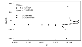
Figure 1: $u<Q(\kappa)>$ versus $\kappa$ for one configuration. $u=2m_{q}$ and $<Q(\kappa)>$ is the average charge density. The unshifted charge (solid dots) has $\kappa_{pole}=.1588539$. The MQA charge (open circles) is smooth (see Section 4).

The existence of isolated poles is obvious. The value of the integrated pseudoscalar charge can be computed, with no appreciable slowdown in convergence, for values of the hopping parameter arbitrarily close to the pole position.

Scans for real poles in the light mass region have now been done for a wide variety of lattice couplings ($\beta=5.5,5.7,5.9,{\rm and}6.1$) and volumes ($8^{3}\times 16,12^{3}\times 24,16^{3}\times 32$ and $24^{3}\times 48$) with both unimproved and $O(a)$ improved Wilson fermions. The frequency of poles versus $\beta$, volume, and quark mass is in generally good agreement with expectations from QED2. For example, at $\beta=5.5$ on a $8^{3}\times 16$ lattice with $O(a)$ improved Wilson fermions ($c_{SW}=1.67$), 255 poles were found in 500 configurations. The distribution of poles for this case is shown in Figure 2.

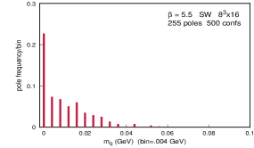
Figure 2: The frequency of poles in the quark propagator versus quark mass. The results use SW fermions on a $8^{3}\times 16$ lattice with $\beta=5.5$. Analysis done by Jim Simone (unpublished).

A detailed study was performed on a sample of 50 gauge configurations on a $12^{3}\times 24$ lattice at $\beta=5.9$ available from the ACPMAPS library [13]. We determined eigenvalues for both the standard Wilson-Dirac action and a Clover action with a clover coefficient of $C_{SW}=1.91$. Six configurations were found with visible poles for each choice of fermion action. These results are shown in Table I. Only one gauge configuration is in common between the two sets of visible poles.

The direct relationship between a nearby pole in the quark propagator and an exceptional configuration at a given quark mass is graphically demonstrated in Figure 3. There the time variation of all 50 pion propagators for $\kappa_{q}=\kappa_{\bar{q}}=0.1595$ is shown. The configurations already identified in Table 1 as having a pole in the visible region are indicated with open circles. The pion propagator is “exceptional” if and only if the configuration has a visible pole in Table 1. Furthermore, the most exceptional configuration (132) has its visible pole at $\kappa=0.1594870$ closest to $\kappa=0.1595$.

As the fermion action is varied, the real eigenvalues move. Therefore, the visible poles, and the corresponding identification of exceptional configurations is a sensitive property of the fermion action and not a property unique to the particular gauge configuration. For example, a small change in the clover coefficient may remove a visible pole for one configuration and add a visible pole for another configuration, completely changing identification of the exceptional configurations. Since only a collision of two real modes allows the pairing required to move off the real axis, small changes in the parameters of the fermion action should not change the number of isolated real modes but only their visibility.

Table 1: Visible poles for a set of 50 gauge configurations.

Wilson Action
Conf.	$\kappa_{pole}$	PS residue
114000	0.1588539	-2.1463
132000	0.1594870	-2.4800
148000	0.1593216	-3.6325
160000	0.1593803	-2.8494
182000	0.1593803	+2.5036
194000	0.1595557	-5.3055

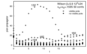
Figure 3: Pion propagators for $\kappa=.1595$ showing all 50 configurations. Visible poles (open circles) and all others (solid dots).

4 The Modified Quenched Approximation

Since the effects of the fermion loop determinant are ignored in the quenched approximation, this approximation is very sensitive to singularities of the fermion propagator which may be encountered in particular formulations of lattice fermions. In particular, the eigenvalue spectrum of Wilson-Dirac fermions generally contains a number of isolated real eigenvalues. In the continuum limit, these eigenvalues are identified as zero modes and occur at precisely zero fermion mass. In the Wilson-Dirac formulation, these eigenvalues shift due to the chiral symmetry breaking generated by the Wilson-Dirac action. Some of these eigenvalues are shifted to positive mass which causes singular behavior for the fermion propagators computed for a mass near a shifted eigenvalue. In the quenched approximation, the shifts cause poles in the fermion propagators which are not properly averaged. This effect corresponds to similar situations in degenerate perturbation theory where small perturbative shifts can cause large effects due to small energy denominators. In this case it is known that it is essential to expand around the exact eigenvalues and compensate the perturbation expansion with counter-terms in each order. In the present case, a similar compensation must be made when using Wilson-Dirac fermions.

We are now able to devise a procedure for correcting the fermion propagators for the artifact of the visible shifted poles. Consider the fermion propagator as a sum over the eigenvalues of the Wilson-Dirac operator (Eq.8). The shifted real eigenvalues cause poles at particular values of the hopping parameter. The residue of the visible poles can be determined by computing the propagator for a range of kappa values close to the pole position and extracting the residue for the full propagator. With this residue we can define a modified quenched approximation by shifting the visible poles to $\kappa=\kappa_{c}$ and adding terms to compensate for this shift. Although simply shifting visible poles to $\kappa_{c}$ would correct for the leading effects, it may distort an ensemble average. Since we are only able to identify poles with positive mass shifts, we have compensated a visible pole with one shifted to negative mass. These negative shifts do not generate singularities in the fermion propagators computed for positive mass values and are expected to cancel against poles with negative shifts generated by other configurations in the ensemble. With this procedure, we do not expect any large renormalization of $\kappa_{c}$ due to the shifting procedure.

The full MQA fermion propagator may be simply computed by adding a term to the naive fermion propagator which incorporates a compensated shift of the visible poles. The modified propagator is given by

$$S^{MQA}(x,y;\{U(A)\})\equiv S(x,y;\{U(A)\})$$

$$~{}~{}~{}~{}~{}~{}~{}~{}~{}~{}~{}~{}~{}~{}~{}~{}~{}~{}~{}+a_{pole}(\kappa)\times{\rm res}_{pole}(x,y)$$

where

$$a_{pole}(\kappa)\equiv-\frac{1}{u-u_{pole}}+\frac{2}{u}-\frac{1}{(u+u_{pole})}$$ (12)

(At large mass the first two terms in the expansion in $1/u$ are not modified and terms linear in the shifts should average to zero), and

$${\rm res}_{pole}(x,y) \equiv f_{pole}(x,U)\bar{g}_{pole}(y,U)$$

$$= \lim_{u\rightarrow u_{pole}}(u-u_{pole})*S(x,y,\{U\})$$

The residue of each pole is extracted by calculating the propagator at $u_{pole}-\Delta$ and $u_{pole}+\Delta$ with $\Delta\approx 10^{-5}$ where the pole position, $u_{pole}$, has been accurately determined from the integrated pseudoscalar charge measurement.

It is important to note that the artifact is the appearance of visible poles at positive mass, not the existence of small or real eigenvalues. It is only the visibility that we have corrected by appealing to the correct behavior in the continuum limit.

5 Applications

MQA quark propagators may now be used in place of the usual quenched propagators. The suppression of the large fluctuations normally associated with the exceptional configurations greatly reduces the errors associated with the propagation of light quarks. The most sensitive physical quantities are those associated with the chiral limit: the pion propagator, the hairpin calculation for the $\eta^{\prime}$ mass and topological quantities.

We have determined fits to the pion mass, $m_{\pi}$, and coupling amplitudes, $|A_{L}|$ and $|A_{S}|$; using pion propagators computed with the limited statistics of the 50 gauge configurations on a $12^{3}\times 24$ lattice at $\beta=5.9$. We simultaneously fit the three pion two-point correlators LS(local-smeared), SL(smeared-local) and SS(smeared-smeared) to a common pion mass. Each two-point pion correlation function, $G_{\pi\pi}(t)$ has the form:

$$G_{\pi\pi}(t)=|A|^{2}\frac{\cosh(m_{\pi}(T/2-t))}{\cosh(m_{\pi}T/2)}$$ (14)

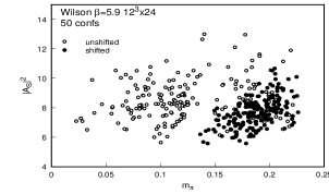
Figure 4: Pion mass, $m_{\pi}$, and smeared coupling amplitude, $|A_{S}|$ for each of 200 bootstrap samples. Naive (open circles) and MQA (solid dots).

We determine fits using 200 bootstrap sets of 50 configurations, In Figure 4, scatter plots compare the fluctuations and correlations for Wilson-Dirac fermions before and after using the MQA analysis for $\kappa=1.590$. It is clear that the MQA analysis greatly reduces the fluctuations and produces a more tightly correlated fit for the mass and decay constant. For the lighter quark masses, it is clear that the normal analysis would not be limited by statistics but by the frequency of exceptional configurations associated with visible poles. However, the MQA analysis cures this problem and higher statistics would now greatly improve the accuracy of computations with light mass quarks.

In Figure 5, we plot the square of the measured values of the pion mass (for the Clover action) against the average of the quark masses, $m_{l}\equiv(m_{q1}+m_{q2})/2$, for the naive and MQA analysis, respectively. The large fluctuations in the naive analysis come when one or both of the quarks are light. The masses determined from the MQA analysis seem to give a good fit to a nearly linear behavior. For general power law form, $m_{\pi}^{2}=A(m_{l}-B)^{C}$, $A=m_{\pi}^{2}/m_{l}=7.45$ and $C\approx 1.1$.

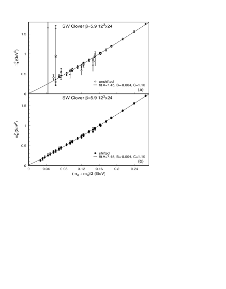
Figure 5: Pion mass plots for Clover action: (a) naive (open circles) and (b) MQA (dots). A power law fit is also shown.

For the naive Wilson action, the slope ($A=m_{\pi}^{2}/m_{l}=4.30$) is in good agreement with previous measurements[13]. The MQA fitted $\kappa_{c}=0.159725$ is very close to the value $\kappa_{c}=0.15972$ obtained from the standard analysis. The small shift in $\kappa_{c}$ reflects our use of a compensated shift for the visible poles and the linearity observed in our mass fits.

A detailed high statistics study on a variety of lattices of these quenched chiral logs as well as the hairpin propagator and associated $\eta^{\prime}$ mass [14]. is underway. Preliminary results indicate that the MQA will allow a direct determination of the power law coefficient, $C=1/(1+\delta)$ in the relation between $M_{\pi}^{2}$ and $m_{l}$ by using very light quark masses.

6 Conclusions

The Wilson-Dirac operator has exact real modes in its eigenvalue spectrum. In the quenched approximation, these real modes can generate unphysical poles in the valence quark propagators for physical values of the quark mass. These poles can produce large lattice artifacts and are the source of the exceptional configurations observed in attempts to directly study QCD in the light quark limit.

The Modified Quenched Approximation identifies and replaces the visible poles in the quark propagator by the proper zero mode contribution, compensated to preserve proper ensemble averages. All usual physical quantities can be computed with only a modest overhead cost required to apply the full MQA analysis. It allows stable quenched calculations with very light quark masses and reduces the errors even in the case of heavier quark mass. Exceptional configurations are eliminated and hence errors can be meaningfully reduced by using larger statistical samples.

The usual O(a) improvement program does not remove the problem of visible poles and exceptional configurations. Indeed, we find the same size spread of the real eigenvalues for both Wilson-Dirac and Clover actions at the same lattice spacing. This suggests the MQA analysis may be an essential ingredient in realistic applications of improved actions on coarse lattices.

Resolving the problem of exceptional configurations removes a major obstacle to studying quenched lattice QCD with Wilson fermions in the light quark limit.

References

- [1] K.-H. Mutter, Ph. De Forcrand, K. Schilling and R. Somer, in Brookhaven 1986, Proceedings, Lattice Gauge Theory, ’86, pg. 257.
- [2] S. Itoh, Y. Iwasaki and T. Yoshie, Phys. Lett. B184 (1987)375; S. Itoh, Y. Iwasaki and T. Yoshie, Phys. Rev. D 36 (1987) 527.
- [3] Y. Iwasaki, Nucl. Phys. B (Proc. Suppl.) 9 (1989)254.
- [4] B.Sheikholeslami and R.Wohlert, Nucl. Phys. B259 (1985) 572; G. Heatlie, G. Martinelli, C. Pittori, G. C. Rossi and C. T. Sachrajda, Nucl. Phys. B352 (1992) 266.
- [5] W. Bardeen, A. Duncan, E. Eichten, G. Hockney and H. Thacker, Fermilab-PUB-97/121-T (1997) (hep-lat/9705008).
- [6] W. Bardeen, A. Duncan, E. Eichten and H. Thacker, Fermilab-PUB-97/119-T (1997) (hep-lat/9705002); A. Duncan (these proceedings).
- [7] T. Banks and A. Casher, Nucl. Phys. B171 (1980) 103.
- [8] Pierre van Baal (these proceedings) and the references therein.
- [9] J. Smit and J. Vink, Nucl. Phys. B286 (1987)485.
- [10] J. Smit and J. Vink, Nucl. Phys. B284 (1987) 234; J. Vink, Nucl. Phys. B307 (1988) 549.
- [11] R. Setoodeh, C.T.H. Davies and L.M. Barbour, Phys. Lett. B213 (1988)195. L. M. Barbour et al., Phys. Rev. D 46 (1992) 3618; J.J.M Verbaarschot, Nucl. Phys. (Proc. Suppl.) B53 (1997) 88.
- [12] Y. Kuramashi, M. Fukugita, H. Mino, M. Okawa and A. Ukawa, Phys. Rev. Lett. 72 (1994)3448.
- [13] A. Duncan, E. Eichten, J. Flynn, B. Hill, G. Hockney and H. Thacker, Phys. Rev D 51 (1995) 5101.
- [14] H. Thacker (these proceedings).