The string tension in SU(N) gauge theory from a careful analysis of smearing parameters.

Abstract

We report a method to select optimal smearing parameters before production runs and discuss the advantages of this selection for the determination of the string tension.

1 Motivation and Introduction

Even though computer power rises it is important to perform the measurements and the data analysis in an optimal way. In the case of the string tension this means that we want to gain maximum information from Wilson loop measurements in minimal time. The smearing procedure proposed by Albanese et al.[1] is an important contribution in this direction.

In principle everything is clear. Select smearing parameters, produce data and analyse/extract the string tension. But what smearing parameters to choose? Measuring a wide range of smearing parameters is expensive; but does it improve the result?

We wanted one set of smearing parameters per coupling to keep CPU costs as low as possible.

Focused on the long distance string behaviour of the potentials measured,we face two problems in the analysis: which local potential to take and which fit ansatz to the potential gives us the string tension?

We show that in each of the steps towards the string tension choices and systematic errors made in the analysis can significantly change the value of the string tension without increasing the statistical error correspondingly. This results in small statistical errors but large systematical errors, that are difficult even to estimate.

We propose a standard procedure, based on physical arguments that minimizes these systematical errors. We have tested this method for different $\beta$, dimension, group, improvement e.g. 1x2, 1x2 with tadpole and also with fermions, but for simplicity here all our results are shown for $\beta=14$ in 3d pure gauge SU(3).

One general remark: Smearing as proposed in [1] improves the signal to noise ratio significantly and does not affect the value of $\sigma$, iff the same parameters are applied to the Wilson loops at given $R$ and to all configurations.

2 Smearing

The smearing procedure replaces a spatial link with a sum of the link and $\epsilon$ times it’s spatial staples. This is applied to all links on the lattice and repeated $n$ times.

As test operator to fix $n$ and $\epsilon$, we selected the loop $W(R=N_{\tau}/2,T=1)={\rm T}(n,\epsilon)$, because we found this Wilson loop maximal improved (lifted “from noise”).

For a given coupling $\beta$ we examine T$(n,\epsilon)$ for $n=1,...40$ and $\epsilon=0.02,...1.0$.

Figure 1. Test operator T$(n,\epsilon)$ vs. n and $\epsilon$ with the isolines of 90%, 95% and 97.5% of maximal improvement.

From figure 1 we see that we reach 97.5% of the maximal possible signal with a set of smearing parameters: $n=10,\epsilon=0.2$ for this $\beta$. One should keep in mind that this figure is different for different values of $\beta$, dimension, group, improvement and fermions. Scanning over a larger area of $n$ and $\epsilon$ we find the isolines closed. Smearing to much can make the signal worse than before.

3 Potential

The local potential $V_{T}(R)$

$$V_{T}(R)=\log\frac{\langle{\rm W}(R,T)\rangle}{\langle{\rm W}(R,T+1)\rangle},$$ (1)

gives the potential $V(R)$ in the limit of large $T$

$$V(R)=\lim\limits_{T\rightarrow\infty}\;V_{T}(R).$$ (2)

Because the local potential approaches the asymptotic value exponentally, we will find significantly different potentials, depending on whether one assumes that asymptotic behaviour sets in at $T=2,3$ or 4.

Figure 2: Potentials $V(R)$ from different local potentials.

In figure 2 we plot smeared and unsmeared potentials for $\beta=14$ in 3d SU(3). The notation $V_{T=2}$ means that the value for the potential $V(R)$ is taken from the $V_{T=2}(R)$. The unsmeared potentials decrease with increasing T. Even $V_{T=3}(R)$ is remarkingly higher than both smeared potentials. The next potential taken from $V_{T=4}(R)$ vanishes at long distance in noise. (In [5] we show that similar effects are observed, if the potential is smeared, but sub optimal smeared.) The smeared potentials are the same within errors, but there too, $V_{T=2}(R)$ is lower (For $T\geq 3$ smeared potentials are the same but errors grow). For the fit we take the lowest, smeared $V_{T}(R)$, typically T = 2 or 3.

4 Fit

In (2+1) dimensions the coulombic force is logarithmic.

$$V_{fit}=V_{0}-\alpha\log R+\sigma R.$$ (3)

Fits to this ansatz are unstable especially for large R. This suggests that because of confinement there is no long range coulombic content in the potential.

We then instead make the Ansatz:

$$V_{fit}=V_{0}-\alpha/R+\sigma R.$$ (4)

This is motivated by the existence of a string fluctuation term $\frac{\pi(D-2)}{24R}$ [2]. We fix $\alpha$ to the corresponding value and make fits from moderate R$(=R_{min})$ to $R=N_{\sigma}/2$. Letting $\alpha$ free and find $\alpha\geq\frac{\pi(D-2)}{24}$ and the string tension from these fits larger than the above.

Figure 3: $\sigma$ vs $R_{min}$ from the fits to formula 4

In figure 3 we plot the string tensions for different fit ranges for free and fixed $\alpha$ fits. We see clearly that unsmeared potentials result in unstable and increasing $\sigma$ for long distance fits. The $\sigma$ for smeared potentials are stable and the same within errorbars for all fits $R_{min}>3$, if $\alpha$ is fixed and only one standard deviation from each other, if $\alpha$ is free. As we want to extract the long distance behaviour, we take $\sigma$ from the fit with $R_{min}=4$ or $5,6,7$.

Scaling of the string tension

In 3d we then plot $\beta\sigma$ versus $1/\beta$ and make a linear or quadratic fit to these points. With these fits we calculate e.g. $T_{c}/\sqrt{\sigma}$ at $\beta_{c}(N_{\tau},N_{\sigma}=\infty)$ [5].

5 Results: $T_{c}/\sqrt{\sigma}$ in 3d and 4d

5.1 3d

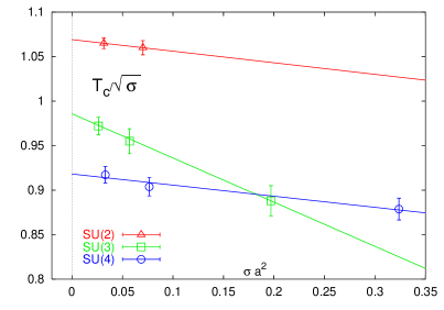
Figure 4: $T_{c}/\sqrt{\sigma}$ in 3d for SU(N), N=2, 3 and 4. The extrapolations to continuum are linear fits in $\sigma a^{2}$.

Our investigation is precise enough to clearly see that the SU(2), SU(3) and SU(4) continuum values differ significantly. For SU(2) earlier results from M. Teper are of the same order but larger [7]. SU(3) meets within errors the prediction (0.977) of the Nambu-Goto string model[3]. SU(2) and SU(4) are only qualitativly similar to the string model prediction.

5.2 4d

Figure 5: $T_{c}/\sqrt{\sigma}$ in 4d for SU(3).The extrapolations to continuum are linear fits in $\sigma a^{2}$.

In figure 5 we show our pure Wilson, 1x2, 1x2 tadpole and 2x2 improved action results. In addition we plot our fits to the potentials published by Iwasakiet al.[4], labeled “RG Improved Tsukuba”. Contrary to Iwasaki et al. we fit the potentials with fixed $\alpha$ and large $R_{min}$, this results in a larger $\sigma$, therefore lower $T_{c}/\sqrt{\sigma}$.

A problem in (3+1) dimensions is, that both string fluctuation term and coulomb forces have $1/R$ shape. A coulombic behaviour can not be ruled out for long distances as easily as in 2+1 dimensions. We find in fits to formula 4 that $\alpha$ is more consistent with a string fluctuation term, because $\sigma$ becames more stable and less dependent from the fit range choosen.

Conclusions:

If we apply the same analysis scheme to all actions, the continuum extrapolations of $T_{c}/\sqrt{\sigma}$ from our data are the same within errors.

In this analysis scheme the continuum string tensions from our fits to the potential data from Iwasaki et al. and our calculations then differ only by one standard deviation.

The work has been supported by the DFG under grants Pe 340/3-3 and Pe 340/6-1.

References

- [1] M. Albanese et al., Phys.Lett.192B:163, 1987
- [2] M. Lüscher, Nucl.Phys.B180:317, 1981
- [3] P. Olesen, Phys.Lett.160B:408, 1985
- [4] Y. Iwasaki et al., Phys.Rev.D56:151-160, 1997
- [5] C. Legeland et al., in preparation
- [6] B. Beinlich et al., hep-lat/9707023
- [7] M. Teper, Phys.Lett.313B:417, 1993 and references therein