Weak matrix elements: On the way to $\Delta I=1/2$ rule and $\varepsilon^{\prime}/\varepsilon$ with staggered fermions.

Abstract

We report progress in our study of hadronic weak matrix elements relevant for the $\Delta I=1/2$ rule and $\varepsilon^{\prime}/\varepsilon$. The presented results are from our first runs on a quenched ensemble with $\beta=6.0$, and a dynamical $N_{f}=2$ ensemble with $\beta=5.7$, using staggered gauge-invariant tadpole-improved fermionic operators.

1 Introduction

An important contribution of Lattice QCD to phenomenology is a first-principle calculation of non-perturbative matrix elements (ME’s) of weak operators involving light hadrons. Knowledge of these ME’s combined with experimental data translates directly to constraints on CKM matrix elements, and thus enables another test of the Minimal Standard Model.

In this work we concentrate on weak decays of kaons into two pions. $\varepsilon^{\prime}$ is the measure of direct CP violation in these decays. It is defined as $\varepsilon^{\prime}=i\mbox{Im}A_{2}e^{i(\delta_{2}-\delta_{0})}/\sqrt{2}A_{0}$, where $A_{2}$, $\delta_{2}$, $A_{0}$ and $\delta_{0}$ are amplitudes and final interaction phases corresponding to isospin 2 and 0 final pion state. New experiments will soon measure $\varepsilon^{\prime}$, hopefully resolving the currently muddy situation. In addition to calculating $\varepsilon^{\prime}$, it is interesting whether Lattice QCD can adequately explain the dominance of $\Delta I=1/2$ transitions in kaon decays, i.e. the fact that $\omega\equiv\mbox{Re}(A_{0}/A_{2})=22.2$.

2 Method

We work within the framework of an effective field theory obtained by integrating out W-boson and t-quark, using OPE and running down the effective Hamiltonian to scales of order of the lattice scale using RG equations [4]. At these scales the effective Hamiltonian has the form

$$H_{W}^{\it eff}=\frac{G_{F}}{\sqrt{2}}V_{ud}\,V^{*}_{us}\sum_{i=1}^{10}\Bigl{[}z_{i}(\mu)+\tau y_{i}(\mu)\Bigr{]}O_{i}(\mu)\,,$$ (1)

where $\tau=-V_{td}V_{ts}^{*}/V_{ud}V_{us}^{*}$, $z_{i}$ and $y_{i}$ are Wilson coefficients (currently known at two-loop order), and $O_{i}$ is the basis of 10 four-fermions operators. In this effective theory $\varepsilon^{\prime}$ can be expressed in terms of CKM matrix elements and $\langle\pi\pi|O_{i}|K\rangle$. Calculating the long-distance part of these ME’s is the task for lattice theorists.

It happens that the value of $\varepsilon^{\prime}$ is dominated by competing contributions of the following two operators:

$$O_{6} = (\bar{s}_{\alpha}d_{\beta})_{V-A}\sum_{q}(\bar{q}_{\beta}q_{\alpha})_{V+A}$$ (2)

$$O_{8} = \frac{3}{2}(\bar{s}_{\alpha}d_{\beta})_{V-A}\sum_{q}e_{q}(\bar{q}_{\beta}q_{\alpha})_{V+A}$$ (3)

In this talk we concentrate mostly on calculation of ME’s involving $O_{6}$.

In general, we follow the technique of calculating ME’s with staggered fermions developed in Ref. [1]. This method has proved to be successful in the past in calculation of the $B_{K}$ parameter, which enters the expression for indirect CP-violation parameter $\epsilon$. Shown in Fig. 1 are our latest results. During the last year, a new point at $\beta=6.4$ has been added. The lattice spacings are determined by demanding asymptotic scaling, with the overall scale taken from the continuum limit of the $\rho$ mass. The final result is $B_{K}(NDR,2{\rm GeV})=0.552\pm 0.007$.

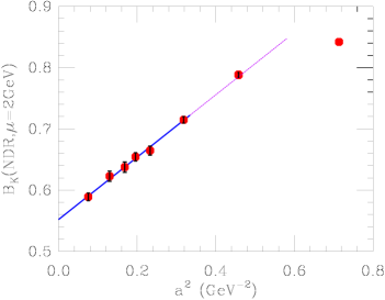
Figure 1: Quenched $B_{K}$ using tadpole improved, gauge-invariant operators.

We would like to achieve similar precision and finesse with much noisier ME’s relevant for $\Delta I=1/2$ rule and $\varepsilon^{\prime}$. We introduce a number of improvements compared to the original work on these ME’s [2].

Due to technical complications, it is extremely difficult to extract four-point functions on the lattice. Instead, we calculate $\langle\pi|H_{W}|K\rangle$ and $\langle 0|H_{W}|K\rangle$ and (following Ref. [3]) use chiral perturbation theory to relate them to $\langle\pi\pi|H_{W}|K\rangle$.

It is convenient to calculate B-ratios of ME’s, which are defined as ratios of ME’s to their values obtained by vacuum saturation. We have to consider three types of 4-fermion contractions: ‘figure-eight’, ‘eye’ and ‘annihilation’. The latter two are notoriously noisy. See Ref. [1] for more details.

3 Simulation

Table 1: Simulation parameters

$\beta$	$N_{f}$	# conf.	Lattice size	$a^{-1}$,GeV	Generated by
6.0	0	216	$16^{3}\times(32\times 4)$	2.1	OSC
5.7	2	71	$16^{3}\times(32\times 4)$	2.0	Columbia

Our simulation parameters are shown in Table 1. We use periodic boundary conditions, and replicate the lattice by a factor of 4 in the time direction. Only degenerate mesons ($m_{s}=m_{d}=m_{u}$) are considered. We employ gauge-invariant, tadpole-improved staggered fermion operators.

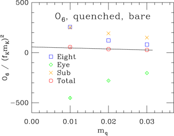
Figure 2: Chiral plot of ME involving $O_{6}$ operator for quenched ensemble, without perturbative corrections. Three contributions come from ‘figure-eight’, ‘eye’ and ‘annihilation’ contractions.

In Fig. 2 we show three contributions to the (bare) ME of $O_{6}$ on a chiral plot. Although individual contributions to $O_{6}$ might be diverging in chiral limit, their sum total seems to converge to a finite value with linear dependence on $m_{q}$, in agreement with chiral symmetries of staggered fermions.

4 Matching with continuum

To quote continuum results we use the ‘horizontal’ matching procedure: using $g_{\overline{MS}}$ as our renormalized coupling constant, we perform the matching to continuum at a scale $q^{*}$ with one-loop perturbation theory [5, 6]:

$$\displaystyle O_{i}^{\it cont}(q^{*})= O_{i}^{\it lat}+\displaystyle\frac{g^{2}(q^{*}a)}{16\pi^{2}}\displaystyle\sum_{j}(\gamma_{ij}\ln(\frac{q^{*}a}{\pi})$$ (4)

$$+C_{ij})O_{j}^{\it lat}+O(g^{4})+O(a^{n})$$

and then run to a specified final scale $\mu$ (e.g. 2 GeV) using continuum two-loop equations. We work in NDR variant of $\overline{\mbox{MS}}$ scheme.

The finite coefficients $C_{ij}$ are uncomfortably big for some operators. In fact, for operators of type $PP$ the perturbative correction is almost the size of the tree-level value. This makes one-loop perturbation theory unreliable. Directly related to this is a huge dependence on $q^{*}$, which serves as an estimate of the size of second-order corrections.

The situation can be made slightly better if we follow the continuum convention and quote results in terms of a $B$ parameter. While there are still potentially large perturbative corrections, we can minimize their effect by considering the $B$ parameter for the operator $O_{6}/Z_{P}^{2}$. This choice modifies both the matching and anomalous dimension matrices, removing the largest corrections from the dominant $PP$ matrix elements, at the expense of larger corrections in front of subdominant operators. As shown in figure 3, the remaining $q^{*}$ dependence is then modest.

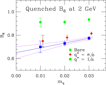
Figure 3: $B_{6}$ ratio for quenched ensemble. The three groups of points correspond to bare operators, and those renormalized in NDR scheme at 2 GeV using two different values for $q^{*}$.

Of course, this sleight of hand doesn’t solve the remaining problem, which is the apparent breakdown of perturbation theory for the pseudoscalar renormalization $Z_{P}$, or equivalently, the quark mass renormalization. Once this coefficient is found (e.g. non-perturbatively) the value of $O_{6}$ will be readily available. The situation with other operators is the same.

For the operators $SS_{1}$, $SS_{2}$ and $PP_{1}$ the renormalization coefficients are not yet known. For the central values we have therefore taken the coefficients appropriate for Landau gauge operators. Varying their values by 100% we find that the change in $B_{6}$ and $B_{8}$ is insignificant. For other operators (namely $B_{5}$ and $B_{7}$) we will eventually need to determine the missing perturbative coefficients.

5 Results and conclusions

Our preliminary results for $B_{6}(\mbox{NDR, 2 GeV})$ at given values of $\beta$ are $0.67\pm 0.04\pm 0.05$ for quenched and $0.76\pm 0.03\pm 0.05$ for dynamical ensembles (first error is statistical, the second one is an estimate of higher-order perturbative corrections). For $B_{8}^{3/2}(\mbox{NDR, 2 GeV})$ we find $1.082\pm 0.006\pm 0.011$ for quenched and $1.12\pm 0.02\pm 0.01$ for dynamical ensembles, in reasonable agreement with results using Landau gauge and smeared operators [7].

We do see a dominance of $\Delta I=1/2$ transition over $\Delta I=3/2$ one. The ratio of amplitudes varies sensitively with the quark mass, but at $ma=.01$, our preliminary results are: $\omega\equiv\mbox{Re}A_{0}/A_{2}=11\pm 1\pm 3$ for quenched and $\omega=16\pm 3\pm 3$ for dynamical ensemble.

We have made a first step in a program to calculate $\varepsilon^{\prime}$ and $\Delta I=1/2$ rule on the lattice. Apart from the common Lattice QCD problems of (partial) quenching, finite lattice spacing and size and degenerate quark masses, we have to face two more problems: failure of perturbation theory, and mostly unknown uncertainty in chiral perturbation theory predictions. To solve the first problem, a non-perturbative determination of $Z_{P}$ is needed. We plan to repeat the calculations for a number of different $\beta$’s in order to take the continuum limit.

We thank the Columbia group for access to the dynamical gauge configurations, and the Ohio Supercomputer Center for the necessary Cray-T3D time.

References

- [1] S. Sharpe, A. Patel, R Gupta, G. Guralnik, G. Kilcup, Nucl. Phys. B 286 (1987) 253-292.
- [2] G. Kilcup, Nucl Phys. B (Proc. Suppl.) 20 (1991) 417-428 (Lattice 1990).
- [3] C. Bernard et al., Phys. Rev. D 32 (1985) 2343.
- [4] A. Buras et al., hep-ph/9303284, Nucl. Phys. B 408 (1993) 209-285.
- [5] S. Sharpe, A. Patel, Nucl. Phys. B 417 (1994) 307-356.
- [6] N. Ishizuka, Y. Shizawa, Phys. Rev. D 49 (1994) 3519-3539.
- [7] G. Kilcup, R. Gupta and S. Sharpe, hep-lat/9707006.