DIMENSIONAL REDUCTION AND HOT QCD: CALCULATING THE DEBYE MASS NON-PERTURBATIVELY

Abstract

We study the phase diagram of the 3-dimensional SU(2) + adjoint Higgs theory, and investigate to what extent it can be used as an effective theory of the 4-dimensional high-$T$ SU(2) QCD. The relation between the parameters in 4 and 3 dimensions is obtained through dimensional reduction. The high-$T$ (deconfined) QCD phase corresponds to the symmetric phase of the 3-D Higgs theory. In the relevant parameter region the symmetric phase is not stable, but the metastability is strong enough to make precise measurements possible. In particular, we measure the Debye mass using a gauge invariant operator.

Numerical lattice Monte Carlo studies of finite temperature QCD are very costly due to the difficulty of the fermionic action simulations. Nevertheless, the effects of fermions are essential at high $T$ and cannot be ignored.[1] This problem can be partly overcome with the dimensional reduction (DR) [2]${}^{\!-\,}$[8]: it provides a method for obtaining an effective 3D bosonic theory for the full 4D finite $T$ QCD. The 3D theory can be derived perturbatively without the infrared problems associated with the standard high-$T$ perturbative analysis. It retains the essential infrared physics of the original theory, and since it is bosonic, it can be studied very economically with lattice Monte Carlo simulations. Recently it has been successfully applied to the Electroweak phase transition.[9]

In this paper we apply DR to SU(2) QCD, and in particular we determine the ${\cal O}(g^{2}T)$ correction to the Debye screening mass in the deconfined phase. This is not computable in perturbation theory.[10]${}^{\!,\,}$[11]

The dimensionally reduced effective theory of the 4D SU(2) QCD with $N_{f}$ fermions is a 3D SU(2) + adjoint Higgs theory:

$$S_{3}=\int\!d^{3}x\biggl{\{}{\frac{1}{4}}F_{ij}^{a}F_{ij}^{a}+{\rm Tr\,}[D_{i},A_{0}][D_{i},A_{0}]+{m_{D}^{2}}{\rm Tr\,}A_{0}^{2}+{\lambda_{A}}({\rm Tr\,}A_{0}^{2})^{2}\biggr{\}}$$ (1)

The Higgs field $A_{0}$ is a remnant of the temporal gauge fields and belongs to the adjoint representation of SU(2). The dimensional reduction is performed at 2-loop level for the couplings $m_{D}^{2}$ and $\lambda_{A}$, and at 1-loop level for the 3D gauge coupling $g_{3}^{2}$ (for details, see [8]). The couplings are dimensionful, and it is convenient to re-express them as a one dimensionful scale and two dimensionless parameters $x$, $y$:

$$g_{3}^{2},~{}~{}~{}y\equiv\frac{m_{D}^{2}}{g_{3}^{4}},~{}~{}~{}x\equiv\frac{\lambda_{A}}{g_{3}^{2}}\,.$$ (2)

For $N_{f}=0$, the 3D couplings are related to the temperature $T$ (and the 4D gauge coupling $g^{2}(\mu)$, which is evaluated at the optimized scale [8] $\mu\approx 2\pi T$) by

$$g_{3}^{2} = g^{2}T={\frac{24\pi^{2}T}{22\log(6.742T/\Lambda_{\overline{\rm MS}})}}$$ (3)

$$x = {\frac{\lambda_{A}}{g_{3}^{2}}}={\frac{10}{22}}{\frac{1}{\log(5.371T/\Lambda_{\overline{\rm MS}})}}$$ (4)

$$y = {\frac{2}{9\pi^{2}x}}\left(1+{\frac{9}{8}}x\right)$$ (5)

The presence of fermions only modifies the numerical factors in the above equations. Most of our results are from $N_{f}=0$ -case, but measuring the same observables for $N_{f}>0$ would be just equally straightforward.

A very important feature of the action given in Eq. 1 is that it is superrenormalisable : it has only linear 1-loop and logarithmic 2-loop divergences. By calculating the divergent counterterms both in the continuum and on the lattice we obtain a definite set of equations linking the 3D continuum coupling constants ($g_{3}^{2},\,x,\,y$) to the corresponding lattice couplings and the lattice spacing. In particular, the dimensionless coupling $\beta_{G}$, which multiplies the lattice gauge action (plaquette term), is related to the continuum gauge coupling $g_{3}^{2}$ and the lattice spacing $a$ by

$$\beta_{G}={\frac{4}{g_{3}^{2}\,a}}\,.$$ (6)

A detailed discussion of the lattice action and the continuum $\leftrightarrow$ lattice connection is given in ref. [8].

Figure 1: The phase diagram of the 3D SU(2) + adjoint Higgs theory. The plot symbols with error bars are lattice results for $y_{c}(x)$ (extrapolated to $V\to\infty$), and the thick line is a 4th order polynomial fit to the data. The dashed line marks the region where the transition turns into a cross-over. The straight lines are the $y_{4D\to 3D}(x)$ curves for the indicated $N_{f}$ -values (for $N_{f}=0$, the line is given by Eq. 5). The top scale shows the values of $T/\Lambda_{\overline{\rm MS}}$ corresponding to the values of $x$ along $y_{4D\to 3D}(x)$ for $N_{f}=0$ (Eq. 4).

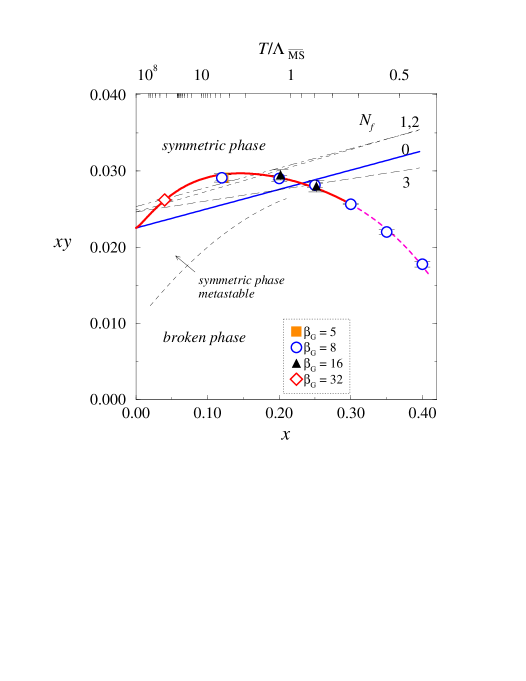
The phase diagram of the SU(2) + adjoint Higgs theory is shown in Fig. 1. For convenience, it is plotted in the ($x,xy$)-plane; the third (dimensionful) coupling $g_{3}^{2}$ gives the length scale. The plot symbols indicate the location of the transition given by the Monte Carlo simulations with different lattice spacings ($\beta_{G}$, Eq. 6). Each of the plot symbols includes a $V\rightarrow\infty$ extrapolation using a series of simulations at finite volumes. The critical curve  $y=y_{c}(x)$ shown is a 4th order polynomial interpolation of the data. Above $y_{c}(x)$ the system is in the symmetric phase, below it in the broken phase. At small $x$, the transition is very strongly first order, but becomes rapidly weaker when $x$ increases. At $x\approx 0.3$–0.33 there is a critical point, after which only a cross-over remains.

The straight lines in Fig. 1 are the ‘dimensional reduction lines’ $y_{4D\to 3D}(x)$ for the number of fermion flavors indicated. The $N_{f}=0$ line is the pure gauge line given in Eq. 5. The 3D theory is well defined on the entire $(x,y)$-plane, but only along $y_{4D\to 3D}(x)$ the 3D theory can describe the physics of the 4D SU(2) gauge theory. Along this line $x$ is related to the temperature as shown on the top axis of the plot (for SU(2), $\Lambda_{\overline{\rm MS}}\approx 1.2T_{c}$ [12]).

Note that in the physically relevant region $T\gg T_{c}\sim\Lambda_{\overline{\rm MS}}$ the physical $y_{4D\to 3D}$ line is in the broken phase .  However, the broken phase cannot describe 4D physics since the perturbative analysis used to derive Eq. 1 is not valid there. Nevertheless, the simulations along $y_{4D\to 3D}(x)$ can still be performed in the symmetric phase: we utilize the fact that due to the strong 1st order nature of the transition at small $x$ the symmetric phase is strongly metastable . The region of metastability is shown with the dashed line in Fig. 1. Excepting microscopic lattice volumes, the system remains in the symmetric phase for the duration of any realistic Monte Carlo simulation.

Figure 2: The Debye mass from operator $h$, in units of $gT$. The line is the 1-parameter fit to Eq. 8.

We measure the Debye screening mass along the $y_{4D\to 3D}(x)$ -line with the operator [10]${}^{\!,\,}$

$$h_{i}=\varepsilon_{ijk}{\rm Tr\,}A_{0}F_{jk}\,.$$ (7)

This operator is the lowest dimensional gauge invariant operator containing only one insertion of $A_{0}$.

When the ${\cal O}(g^{2}T)$ corrections to the Debye mass are included,

$$m_{D}=m_{D,0}+{\frac{g^{2}T}{2\pi}}\log{\frac{m_{D,0}}{g^{2}T}}+C_{2}\,g^{2}T+{\cal O}(g^{3}T)\,,$$ (8)

where $m_{D,0}=\sqrt{2/3}gT$ is the leading order contribution and the coefficient in front of the log-term is a result of a perturbative computation of the pole $A_{0}$ mass.[11] The coefficient $C_{2}$ is not computable perturbatively.

To improve the signal we use recursive smearing and blocking of both the gauge fields and the Higgs field. In order to observe the true asymptotic behavior we use very small values of $x$, which correspond to extremely large $T$ – up to $10^{100}\times T_{c}$.

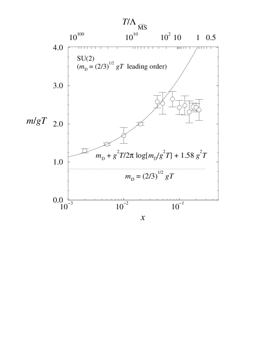
In Fig. 2 we show the data in units of $gT$ along the $y=y_{4D\to 3D}(x)$ -line (for $N_{f}=0$). The temperature in physical units is shown in the top scale of the figure. When $x\mathop{\raise 1.29167pt\hbox{$<$\kern-7.5pt\raise-4.73611pt\hbox{$\sim$}}}0.05$ ($T\mathop{\raise 1.29167pt\hbox{$>$\kern-7.5pt\raise-4.73611pt\hbox{$\sim$}}}100\Lambda_{\overline{\rm MS}}\sim 100T_{c}$) the asymptotic function Eq. 8 fits the data well, with the result

$$C_{2}=1.58\pm 0.18\,.$$ (9)

From Fig. 2 we observe that at all realistic temperatures, the corrections to the leading order result $m_{D,0}$ are very large. $m_{D,0}$ dominates only when $x\mathop{\raise 1.29167pt\hbox{$<$\kern-7.5pt\raise-4.73611pt\hbox{$\sim$}}}0.01$, corresponding to temperatures $T\mathop{\raise 1.29167pt\hbox{$>$\kern-7.5pt\raise-4.73611pt\hbox{$\sim$}}}10^{20}\Lambda_{\overline{\rm MS}}$! Interestingly, when $T\mathop{\raise 1.29167pt\hbox{$<$\kern-7.5pt\raise-4.73611pt\hbox{$\sim$}}}100T_{c}$, the mass remains approximately constant, $m_{D}\sim 3\,m_{D,0}$. Large values for $m_{D}$ have also been observed in 4D SU(2) simulations, using gluon propagators in Landau gauge.[15]

References

- [1] For a review, see A. Ukawa, Nucl. Phys. B (Proc. Suppl.) 53, 106 (1997).
- [2] P. Ginsparg, Nucl. Phys. B 170, 388 (1980).
- [3] T. Appelquist and R. Pisarski, Phys. Rev. D 23, 2305 (1981).
- [4] S. Nadkarni, Phys. Rev. D 27, 917 (1983);Phys. Rev. D 38, 3287 (1988).
- [5] K. Farakos, K. Kajantie, K. Rummukainen and M. Shaposhnikov, Nucl. Phys. B 425, 67 (1994).
- [6] E. Braaten and A. Nieto, Phys. Rev. D 51, 6990 (1995).
- [7] K. Kajantie, M. Laine, K. Rummukainen and M. Shaposhnikov, Nucl. Phys. B 458, 90 (1996).
- [8] K. Kajantie, M. Laine, K. Rummukainen and M. Shaposhnikov, Nucl. Phys. B, in press [hep-ph/9704416].
- [9] For a review, see K. Rummukainen, Nucl. Phys. B (Proc. Suppl.) 53, 30 (1997).
- [10] P. Arnold and L.G. Yaffe, Phys. Rev. D 52, 7208 (1995).
- [11] A.K. Rebhan, Phys. Rev. D 48, R3967 (1993); Nucl. Phys. B 430, 319 (1994).
- [12] J. Fingberg, U. Heller and F. Karsch, Nucl. Phys. B 392, 493 (1993).
- [13] L. Kärkkäinen, P. Lacock, D.E. Miller, B. Petersson and T. Reisz, Nucl. Phys. B 418, 4 (1994).
- [14] A. Hart, O. Philipsen, J.D. Stack and M. Teper, Phys. Lett. B 396, 217 (1997).
- [15] U. Heller, F. Karsch and J. Rank, Proceedings of Lat’97, Nucl. Phys. B, to be published.