PHASE DIAGRAM OF 3D U(1)+HIGGS THEORY

Abstract

We study the properties of the phase transition in three dimensional U(1)+Higgs theory or Ginzburg-Landau model of superconductivity. Special attention is paid to large values of scalar self coupling (Type II superconductors), where the nature of the transition is unclear. We present some evidence for an unusual transition in this regime.

1 Introduction

Three dimensional SU(2)+Higgs theory is an effective theory for the electroweak sector of the Standard Model at high temperatures and therefore can be used to describe the electroweak phase transition.[1] It is interesting to compare how the properties of system change when one replaces the non-abelian gauge group SU(2) with abelian U(1). This results in U(1)+Higgs theory in three dimensions, which is also known as Ginzburg-Landau model.

Ginzburg-Landau model is also an effective theory for describing the superconducting transition between normal and superconducting states. This gives additional motivation for studying the properties of the phase transition in U(1)+Higgs model.

In this talk I describe numerical simulations I have done in collaboration with K. Kajantie, M. Laine and M. Karjalainen.[2]

2 3d U(1)+Higgs theory

The three dimensional U(1)+Higgs theory is a locally gauge invariant continuum U(1) + complex scalar field theory defined by

$$S = \int d^{3}x\biggl{[}\frac{1}{4}(\partial_{i}A_{j}-\partial_{j}A_{i})^{2}+|(\partial_{i}+ie_{3}A_{i})\phi|^{2}+m_{3}^{2}\phi^{*}\phi+\lambda_{3}\left(\phi^{*}\phi\right)^{2}\bigg{]}.$$

This theory contains three dimensionful parameters $(e_{3},m_{3},\lambda_{3})$, so one can factor out one scale. This leaves only two parameters $y\equiv m_{3}^{2}(e_{3}^{2})/e_{3}^{4},\,\,x\equiv\lambda_{3}/e_{3}^{2}$.

It is well known [3] that for small values of $x$ (Type I superconductors) the system has a first order phase transition at some critical point $y_{c}(x)$, but the situation for large values of $x$ (Type II) is less clear. A schematic phase diagram is shown in Figure 1, and the main question we are trying to answer is: how do the properties of the phase transition change when we move from small values of $x$ to large values of $x$?

Figure 1: The qualitative phase diagram of the 3d U(1)+Higgs model

For large values of $x$ the perturbation theory breaks down and one has to use non-perturbative methods to study the system. This can be done by discretizing the system with finite lattice (with lattice spacing $a$). This results in

$$S = \beta_{G}\sum_{\mbox{\bf x},i<j}\{1-\cos[\alpha_{ij}(\mbox{\bf x})]\}-\beta_{H}\sum_{\mbox{\bf x},i}{\mbox{Re}}\,\phi^{*}(\mbox{\bf x})U_{i}(\mbox{\bf x})\phi(\mbox{\bf x}+\hat{i})$$

$$+\sum_{\mbox{\bf x}}\phi^{*}(\mbox{\bf x})\phi(\mbox{\bf x})+\beta_{R}\sum_{\mbox{\bf x}}\left[\phi^{*}(\mbox{\bf x})\phi(\mbox{\bf x})\right]^{2},$$

where $\beta_{G}=1/e_{3}^{2}a$ and $\alpha_{ij}(\mbox{\bf x})=\alpha_{i}(\mbox{\bf x})+\alpha_{j}(\mbox{\bf x}+\hat{i})-\alpha_{i}(\mbox{\bf x}+\hat{j})-\alpha_{j}(\mbox{\bf x})$. The relation between other two lattice parameters can be obtained by relating the counter terms in the $\overline{\mbox{\rm MS}}$ and lattice regularisation schemes.[4]

We focus our studies mainly to the mass spectrum of the system. It turns out that the mass of the lowest vector state ($m_{\gamma}$) serves as an order parameter for the system at continuum limit. However, at finite lattice spacing $a$ this mass cannot be an order parameter. This is due to the fact that we use compact formulation for the gauge field, as it is possible to show [5] that then the monopoles create a mass (which depends on lattice spacing) to this state. A semiclassical calculation can be used to give an estimate for this mass, and we obtain at $\beta_{G}=4$ an extremely small value $m_{\gamma}/e_{3}^{2}=0.003$.

3 Simulations

To study the phase diagram of the system, we have used two values of $x$: one ($x=0.0463$) corresponding to strongly Type I behaviour and one ($x=2$) corresponding to strongly Type II. At both points we use several different lattice sizes and try to work with as small lattice spacing as possible while still keeping the physical size of the system reasonably large.

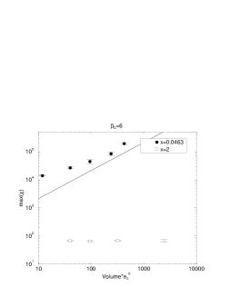
Figure 2: The maximum of the susceptibility of $\phi^{*}\phi$ for Type I and Type II superconductors. The straight line is the expected behaviour in first order phase transition.

As previously mentioned, we concentrate on the masses of the system. We measure three different operators

$$O(\mbox{\bf x}) = \phi^{\ast}(\mbox{\bf x})\phi(\mbox{\bf x}),\,\,\,O_{i}(\mbox{\bf x})=\mathop{\rm Im}\phi^{\ast}(\mbox{\bf x})U_{i}(\mbox{\bf x})\phi(\mbox{\bf x}+\hat{i}),$$

$$O_{ij}(\mbox{\bf x}) = \sin[\alpha_{i}(\mbox{\bf x})+\alpha_{j}(\mbox{\bf x}+\hat{i})-\alpha_{i}(\mbox{\bf x}+\hat{j})-\alpha_{j}(\mbox{\bf x})].$$

The masses we extract from asymptotic behaviour of these operators are labelled $m_{H},m_{W}$ and $m_{\gamma}$ respectively. To enhance the projection of these operators to the ground state we use blocking. This is absolutely essential in order to get a good signal.

In addition to the masses, we measure the susceptibility of operator $\phi^{*}\phi$. Using finite size scaling, it is possible to distinguish between first or higher order phase transitions using this operator. In a first order phase transition, where there are two different phases, the maximum of susceptibility grows linearly with volume $\chi\sim V$. In second order phase transition the expected behaviour is $\chi\sim V^{\alpha}$, where $\alpha$ is a critical exponent of the system. If there is no transition, or the transition is of higher than second order, or the critical exponent $\alpha\leq 0$, the maximum is constant: $\chi\sim V^{0}$.

3.1 Type I

We first discuss the transition at small values of $x$. At this regime we see a very clear two peak structure in $\phi^{*}\phi$. The susceptibility calculated from these data clearly shows linear growth with increasing volume, as can be seen from Figure 2.

Also the mass spectrum of the system shows signal of first order phase transition. From Figure 3 (left) one can see that all masses have a clear discontinuity at critical point; furthermore the vector mass $m_{\gamma}$ drops to zero at critical point $y_{c}$, and is consistent with being zero for $y>y_{c}$. Thus even though not rigorously an order parameter, it can be used as an order parameter for practical purposes.

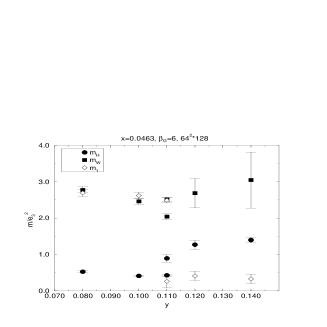
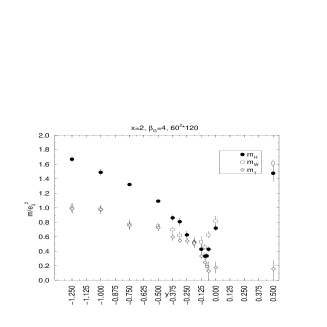
Figure 3: Masses at $x=0.0463$ and at $x=2$.

3.2 Type II

For large values of $x$ the system behaves in strikingly different way. It is obvious from Figure 2 that the maximum of the susceptibility stays constant as one increases volume, which could in principle mean that there is no phase transition as in SU(2)+Higgs.[6] However, as previously stated this cannot be true in the continuum limit, so the transition must either be of second order with critical exponent $\alpha\leq 0$ or of higher order.

If the transition is of second order one would expect that all the masses vanish at the critical point (as the corresponding correlation lengths diverge). We have plotted the three masses we study on Figure 3 (right). One clearly sees that even though the vector mass $m_{\gamma}$ goes to zero at critical point the scalar mass $m_{H}$ (and the exited state of vector mass $m_{W}$) remains finite at $y_{c}$.

There are two possible reasons for $m_{H}$ to stay nonzero even in second order transition. Firstly one should check that we are working with such a large volumes that there are no finite size effects. This is especially important because there are (nearly) massless exitations in the vicinity of the phase transition. We have performed simulations with three different lattice sizes, ranging from $32^{3}$ to $60^{2}\times 120$, and see no systematic evidence for finite size effects.

The second explanation would be that the masses remain nonzero for any finite lattice spacing $a$, but vanish at continuum limit. However, we work with extremely small lattice spacing (near phase transition our typical correlation length for scalar operator $O$ is roughly ten times the lattice spacing) so one would expect that the results do not change significantly when taking $a\to 0$. This is further supported by the fact that the mass of the photon, which is expected to be finite at nonzero lattice spacing, is withing our statistical errors consistent with being zero.

4 Conclusions

We have shown evidence towards a non-typical phase transition at Type II ($x$ large) regime. We find a nonvanishing scalar mass even at pseudo-critical point even though the vector mass vanishes. Thus the vector mass serves as an order parameter for the system. The fact that scalar mass does not vanish means that if the transition is of second order, it is rather atypical. However, as it is possible that the vector mass goes to zero continuously, one cannot exclude the possibility of a second order phase transition.

References

References

- [1] M. Laine, these proceedings [hep-ph/9707415].
- [2] K. Kajantie, M. Karjalainen, M. Laine and J. Peisa, cond-mat/9704056. M. Karjalainen, M. Laine and J. Peisa, Nucl. Phys. B (Proc. Suppl.) 53 (1997) 475-478. M. Karjalainen and J. Peisa, hep-lat/9607023.
- [3] See for example H. Kleinert, Gauge Fields in Condensed Matter, World Scientific, 1989.
- [4] M. Laine, Nucl. Phys. B 451, 484 (1995)
- [5] A. Polyakov, Phys. Lett. B 59, 82 (1975).
- [6] K. Kajantie, M. Laine, K. Rummukainen and M. Shaposhnikov, Phys. Rev. Lett. 77, 2887 (1996) [hep-ph/9605288].