Where the electroweak phase transition ends

Abstract

We give a more precise characterisation of the end of the electroweak phase transition in the framework of the effective $3d$ $SU(2)$–Higgs lattice model than has been given before. The model has now been simulated at gauge couplings $\beta_{G}=12$ and $16$ for Higgs masses $M_{H}^{*}=70,74,76$ and $80$ GeV up to lattices $96^{3}$ and the data have been used for reweighting. The breakdown of finite volume scaling of the Lee–Yang zeroes indicates the change from a first order transition to a crossover at $\lambda_{3}/g_{3}^{2}=0.102(2)$ in rough agreement with results of Ref. [1] at $\beta_{G}=9$ and smaller lattices. The infinite volume extrapolation of the discontinuity $\Delta\langle\phi^{+}\phi\rangle/g_{3}^{2}$ turns out to be zero at $\lambda_{3}/g_{3}^{2}=0.107(2)$ being an upper limit. We comment on the limitations of the second method.

I Introduction

During the last couple of years, big effort has been invested to study the properties of the first order phase transition that the standard model was expected to undergo at high temperature (for reviews see [2]). The motivation was to explore the phenomenological viability of the generation of the baryon asymmetry of the universe at this transition.

The perturbative evaluation of the phase transition is prevented by infrared divergences in the so–called symmetric phase. Lattice Monte Carlo studies of the $4$ dimensional $SU(2)$–Higgs theory [3, 4] have been done so far for relatively large lattice spacings (neglecting the U(1) gauge group and the fermionic content of the theory). Another approach is based on the concept of dimensional reduction [5]. One maps the theory (with or without fermions) onto a $3$ dimensional $SU(2)$–Higgs model containing all infrared problems of the full theory and can investigate this effective theory by Monte Carlo simulations [6, 7, 8, 1] with much less effort. Later, the $U(1)$ gauge group has been included into this approach, too [9].

BAU generation at the phase transition of the standard model is ruled out already, and the primary interest has shifted to extensions of the standard model. Nevertheless, the standard variant remains interesting in order

1. to understand methods like dimensional reduction, validity of perturbation theory etc. in the realm of extremely weakly first order phase transitions and

2. to understand in general terms the physics in the strongly coupled high temperature phase of gauge–matter systems.

The present paper belongs to the first group of studies. We try to shed light on the question for which Higgs mass the first order transition ceases to exist and what replaces it at slightly higher Higgs mass. Analytical work has already addressed this problem. In [10] it has been claimed that the transition between the broken and the symmetric phase can only be of first order or a smooth crossover. Within the same average action approach it has been made more precise later [11] that the first order transition ends at a Higgs mass of about $80$ GeV and the transition is replaced by a unique strongly interacting phase. A similar conclusion has been drawn from a renormalisation group study of the electroweak phase transition [12]. Analysing gap equations a similar critical Higgs mass has been pointed out in Ref. [13].

Recently, $3d$ Monte Carlo studies [14, 1] have investigated the volume dependence of the susceptibility of the Higgs condensate. These studies gave support for the claim that the transition turns into a smooth crossover for large Higgs masses. An attempt to determine the value of the upper critical Higgs mass has been performed in [1]. It was based on an analysis of the volume dependence of the Lee–Yang zeroes [15], but for a relatively large lattice spacing. The exploration of critical behaviour in lattice gauge theories using Lee–Yang zeroes has become a frequently used tool nowadays. A good guide to the basic applications can be found in [16].

The only $4d$ study to determine the critical Higgs mass region has been presented in [17], however with a temporal extent of only $N_{t}=2$ and an exploratory scan of the Higgs self coupling (corresponding to different Higgs masses).

In our present study we use Monte Carlo simulations of the three dimensional theory in order to find the critical Higgs mass, employing two different types of analysis. The first is plainly to look for the Higgs mass where the jump of the scalar condensate (which is proportional to the latent heat) vanishes. The second method is based on an analysis of the Lee–Yang zeroes of the partition function, whose finite volume behaviour changes with the character of the transition and is able to characterise the change of first order into crossover.

II The model and numerical techniques

The lattice $3d$ $SU(2)$–Higgs model is defined by the action

$$S = \beta_{G}\sum_{p}\big{(}1-{1\over 2}{\mathrm{t}r}U_{p}\big{)}-\beta_{H}\sum_{x,\alpha}E_{x,\alpha}$$ (2)

$$+\sum_{x}\big{(}\rho_{x}^{2}+\beta_{R}(\rho_{x}^{2}-1)^{2}\big{)}$$

$$E_{x,\alpha} = {1\over 2}{\mathrm{t}r}(\Phi_{x}^{+}U_{x,\alpha}\Phi_{x+\alpha})$$ (3)

(summed over plaquettes $p$, sites $x$ and directions $\alpha$), with the gauge coupling $\beta_{G}$, the lattice Higgs self–coupling $\beta_{R}$ and the hopping parameter $\beta_{H}$. The gauge fields are represented by unitary $2\times 2$ link matrices $U_{x,\alpha}$ and the Higgs fields are written as $\Phi_{x}=\rho_{x}V_{x}$. $\rho_{x}^{2}=\frac{1}{2}{\mathrm{t}r}(\Phi_{x}^{+}\Phi_{x})$ is the Higgs modulus squared, $V_{x}$ an element of the group $SU(2)$, $U_{p}$ denotes the $SU(2)$ plaquette matrix. For shortness, we characterise as in [8] the Higgs self–coupling by an approximate Higgs mass $M_{H}^{*}$ defined through

$$\beta_{R}=\frac{\lambda_{3}}{g_{3}^{2}}\frac{\beta_{H}^{2}}{\beta_{G}}=\frac{1}{8}{\left(\frac{M_{H}^{*}}{80\ {\mathrm{G}eV}}\right)}^{2}\frac{\beta_{H}^{2}}{\beta_{G}},$$ (4)

where $\lambda_{3}$ and $g_{3}$ are the dimensionful quartic and gauge couplings of the corresponding $3d$ continuum model, respectively. Both couplings are renormalisation group invariants. The $3d$ continuum model is furthermore characterised by the renormalised mass $m_{3}(g_{3}^{2})$ taken at the scale $\mu_{3}=g_{3}^{2}$. To study the continuum limit of the lattice model at given $M_{H}^{*}$ (along the line of constants physics of the $3d$ continuum theory) one has to keep the coupling ratios $\lambda_{3}/g_{3}^{2}$ and $m_{3}(\mu_{3}=g_{3}^{2})/g_{3}^{2}$ fixed.

Letting increase the gauge coupling $\beta_{G}$ at fixed $\lambda_{3}/g_{3}^{2}$ along the critical line dividing the high temperature and Higgs phase ($m_{3}(g_{3}^{2})/g_{3}^{2}$ fixed and near to zero) permits to perform the continuum limit according to the relation

$$\beta_{G}=\frac{4}{ag_{3}^{2}}$$ (5)

We study the phase transition driven by the hopping parameter $\beta_{H}$. The Monte Carlo simulations are performed at $\beta_{G}=12$ and $\beta_{G}=16$ for different $M_{H}^{*}$, ranging from $70$ to $80$ GeV at several values of $\beta_{H}$ on cubic lattices of the size $L^{3}$ (see Table I for parameters and statistics). The simulations have been performed at the DFG Quadrics computer QH2 in Bielefeld and on the CRAY-T90 of the HLRZ Jülich, some data have been collected on a Q4 Quadrics in Jülich. For the update we used the same algorithm as described in [8] which combines Gaussian heat bath updates for the gauge and Higgs fields with several reflections for the fields to reduce the autocorrelations. All thermodynamical bulk quantities are measured after each such combined sweep. One combined sweep with bulk measurements takes $3.5$ sec on a $96^{3}$ lattice on the QH2 parallel computer.

In the search for the phase transition the space averaged square of the Higgs modulus

$$\rho^{2}=\frac{1}{L^{3}}\sum_{x}\rho_{x}^{2}$$ (6)

is used, $\langle\rho^{2}\rangle$ denotes averaging over the Monte Carlo measurements.

In our analysis we have used the Ferrenberg–Swendsen method [18]. Note that at fixed $M_{H}^{*}$ (and $\beta_{G}$) the Higgs self–coupling $\beta_{R}$ is quadratic in $\beta_{H}$ (see Eq. 4). The reweighting has to be performed by histogramming in two parts of the action. The partition function is represented as

$$Z(L,\beta_{H})=$$ (8)

$$\int dS_{1}dS_{2}D_{L}(S_{1},S_{2})\exp\left(L^{3}(\beta_{H}S_{1}-\beta_{H}^{2}S_{2})\right)\ ,$$

$$S_{1}=3E_{\mathrm{l}ink}\ ,\ \ \ S_{2}=\frac{\lambda_{3}}{g_{3}^{2}\beta_{G}}(\rho^{4}-2\rho^{2})$$ (9)

where the density of states $D_{L}(S_{1},S_{2})$ is approximated by the histogram produced by multihistogram reweighting of all available data for given $\beta_{G}$ and $L^{3}$ (see Table I). Having a good estimator of the density of states $D_{L}(S_{1},S_{2})$ from a sufficient number of simulation points we are able to

• interpolate in $\beta_{H}$ at fixed $M_{H}^{*}$ to localise the phase transition,

• interpolate in $M_{H}^{*}$ in order to find the critical Higgs mass,

• extrapolate to complex $\beta_{H}$ to study Lee–Yang zeroes.

Finally, all considered quantities are translated into physical units. This allows to combine results obtained for different $\beta_{G}$ and gives a check to what extent the continuum limit is reached. The size of the lattice in continuum length units (i.e. the inverse $3d$ gauge coupling $g_{3}^{2}$) is given by the expression

$$lg_{3}^{2}=Lag_{3}^{2}=4L/\beta_{G}$$ (10)

and the jump of the quadratic scalar condensate is in the corresponding mass units

$$\frac{\Delta\langle\phi^{+}\phi\rangle}{g_{3}^{2}}=\frac{1}{8}\beta_{G}\beta_{H}\Delta\langle\rho^{2}\rangle\ .$$ (11)

Here $\Delta\langle\rho^{2}\rangle=\langle\rho^{2}_{\mathrm{b}}\rangle-\langle\rho^{2}_{\mathrm{s}}\rangle$ denotes the difference of the lattice quadratic scalar condensates measured at the pseudo–critical hopping parameter between the broken ($\langle\rho^{2}_{\mathrm{b}}\rangle$) and symmetric ($\langle\rho^{2}_{\mathrm{s}}\rangle$) phases, respectively.

III The behaviour of the latent heat with increasing Higgs mass

A non–vanishing latent heat $\Delta\epsilon$ is one of the characteristics for a first order phase transition. In our model the latent heat is proportional to the jump of the quadratic scalar condensate $\Delta\langle\phi^{+}\phi\rangle$ [6]. The proper identification of the scalar condensate discontinuity becomes increasingly demanding near to the end of the first order transition. The correlation length grows beyond the size of the system under study, in particular if the endpoint is a critical point. There can be an apparent metastability on a finite torus which delays the approach to the thermodynamical limit.

In this section we identify the end of the phase transition with the point in the $\beta_{H}$–$M_{H}^{*}$ plane where the discontinuity vanishes.

The minimum of the Binder cumulant

$$B_{\rho^{2}}(L,\beta_{H})=1-{\frac{{\langle({\rho^{2}})^{4}\rangle}}{{\ 3{\langle({\rho^{2}})^{2}\rangle}^{2}}}}$$ (12)

and the maximum of the susceptibility of $\rho^{2}$

$$C_{\rho^{2}}(L,\beta_{H})=\langle({\rho^{2}})^{2}\rangle-\langle{\rho^{2}}\rangle^{2}$$ (13)

are chosen to define pseudo–critical values of the hopping parameter $\beta_{H}$. The jumps in $\Delta\langle\rho^{2}\rangle$ are extracted from the peaks of the histograms reweighted to these values of $\beta_{H}$. The $\rho^{2}$ histograms at the respective pseudo–critical couplings show how the discontinuity decreases with increasing $M_{H}^{*}$. The gap between the peaks is more and more filled, and the distance between them becomes smaller (Fig. 1).

At any Higgs mass $M_{H}^{*}$ we attempt to perform the thermodynamical limit of $\Delta\langle\rho^{2}\rangle$ by assuming the finite size corrections to follow an inverse cross sectional law (suggested by the behaviour of the Potts model in $2$ dimensions [19])

$$\left|\Delta\langle\phi^{+}\phi\rangle_{\infty}-\Delta\langle\phi^{+}\phi\rangle_{l}\right|\propto 1/l^{2}\,.$$ (14)

Fig. 2 shows the different infinite volume extrapolation of $\Delta\langle\phi^{+}\phi\rangle/g_{3}^{2}$ at $M_{H}^{*}=70$ and $76$ GeV. We have used two criteria (minimum of the Binder cumulant and maximum of the susceptibility for the lattice quadratic Higgs condensate) to determine the pseudo–critical $\beta_{H}$. One observes that the data for different $\beta_{G}$ cluster along one curve within their errors and do not show a significant dependence on the lattice spacing $a$. Therefore, we conclude that the quadratic Higgs condensate jump at the measured $\beta_{G}$ values is already sufficiently near to the continuum limit. Obviously the latent heat at $M_{H}^{*}=76$ GeV has a vanishing thermodynamical limit. At the larger Higgs mass the assumed $1/l^{2}$ scaling compatible with the vanishing limit of the condensate sets in only for the largest considered volumes.

This feature becomes even more pronounced at intermediate Higgs mass, $M_{H}^{*}=74$ GeV. Fig. 3 shows the volume dependence of the condensate jump for $M_{H}^{*}=74$ GeV. This picture includes, besides reweighted data, original simulations at that Higgs mass for lattices up to $96^{3}$ at $\beta_{G}=12$. The onset of the $1/l^{2}$–scaling is delayed to lattices not smaller than $80^{3}$ (for $\beta_{G}=12$). If only those data are considered the latent heat is consistent with zero.

The summary of the extrapolations to the thermodynamical limit is collected in Fig. 4. For the extrapolation according to Eq. (14) we have used the results for the discontinuity at $(lg_{3}^{2})^{-2}<0.003$ which correspond to lattices $\geq 64^{3}$ for $\beta_{G}=12$ and $80^{3}$ for $\beta_{G}=16$. For $\lambda_{3}/g_{3}^{2}\approx 0.107$ ($M_{H}^{*}=74$ GeV) a different extrapolation is shown, lying below the general trend, which is compatible with zero at that Higgs mass. This extrapolation takes into account only the two largest volumes at $\beta_{G}=12$. The uncertainty reflects the scattering of slopes of the straight line interpolation.

Concerning the two–parameter multihistogram extrapolation we can report that the purely interpolated histograms at $M_{H}=74$ GeV near to the endpoint are in reasonable agreement with histograms at that mass supported by actual simulations. However, at that mass we are too near to the endpoint, such that simulations at still larger lattices are necessary in order to estimate the correct thermodynamical limit.

We conclude that the critical coupling, if defined by vanishing latent heat (vanishing jump of the quadratic scalar condensate), is bounded from above as

$$\lambda_{3{\mathrm{c}rit}}/g_{3}^{2}<0.107\ .$$ (15)

This bound is somewhat larger than the critical coupling given in [1]. It could be tempting to explain this difference to the somewhat smaller $\beta_{G}=9$ in their paper.

In this section we have assumed an early continuum limit by plotting data from different $\beta_{G}$ as a function of the physical lattice volume. The data were compatible with each other within the errors. The account for finite $a$ corrections of expectation values in the thermodynamical limit could be performed (if necessary) along the line of Ref. [20].

IV Lee–Yang zeroes near the critical Higgs mass

In this section we will determine the critical Higgs mass by analysing the position of the Lee–Yang zeroes in the complex $\beta_{H}$ plane and their motion with increasing size of the finite lattice system.

Phase transitions correspond to non–analytical behaviour of the infinite volume free energy density as function of couplings which normally are real–valued. This is signalled by zeroes in the complex plane (to which the relevant coupling constant is extended) of the partition function of finite systems. If there exists a phase transition driven by this coupling some of these zeroes cluster, in the thermodynamical limit, along lines that pinch the real axis. This prevents the analytic continuation along the real axis corresponding to that coupling.

We sketch here the motion of the most important zeroes with increasing volume. Neglecting interface tension effects the partition function at the transition point is given by the contributions of the two phases

$$Z=Z_{s}+Z_{b}=e^{-L^{3}f_{s}}+e^{-L^{3}f_{b}}$$ (16)

where $f_{s(b)}$ denotes the lattice free energy per site of the so–called symmetric (broken) phase. The free energy density can be expanded around the real–valued pseudo–critical coupling $\beta_{Hc}$

$$f_{s,b}(\beta_{H}) = f(\beta_{Hc})+\langle E_{s,b}(\beta_{Hc})\rangle(\beta_{H}-\beta_{Hc})$$ (18)

$$+{\cal O}((\beta_{H}-\beta_{Hc})^{2})\ .$$

To obtain $\langle E\rangle$ we use the action in the form

$$S=S_{0}-3\beta_{H}L^{3}E_{\mathrm{l}ink}+\beta_{R}^{2}L^{3}(\rho^{4}-2\rho^{2})$$ (19)

with $\rho^{2}$ defined in Eq. (6) and

$$E_{\mathrm{l}ink}=\frac{1}{3L^{3}}\sum_{x,\alpha}E_{x,\alpha}\ ,\ \ \ \rho^{4}=\frac{1}{L^{3}}\sum_{x}\rho_{x}^{4}\ .$$ (20)

Taking into account that the Higgs self–coupling is (for given $M_{H}^{*}$) quadratic in $\beta_{H}$ we find

$$\langle E(\beta_{Hc})\rangle=-3\langle E_{\mathrm{l}ink}\rangle+2\frac{\beta_{Rc}}{\beta_{Hc}}\left(\langle\rho^{4}\rangle-2\langle\rho^{2}\rangle\right)$$ (21)

where $\langle\dots\rangle$ denotes the Monte Carlo average as before.

Using the decomposition at $\beta_{Hc}$

$$\langle E_{s(b)}\rangle=\langle E\rangle\mp\frac{1}{2}\Delta\langle E\rangle\ ,$$ (22)

the partition sum behaves as

$$Z\propto\cosh\left[\frac{\Delta\langle E\rangle}{2}L^{3}(\beta_{H}-\beta_{Hc})\right]\ .$$ (23)

For the complex coupling $\beta_{H}={\mathrm{R}e}\beta_{H}+i~{}{\mathrm{I}m}\beta_{H}$ we obtain in this approximation that the zeroes of the complex partition function $Z$ are located at ($n$ are integers)

$${\mathrm{I}m}\beta_{H}^{(n)} = \frac{2\pi}{L^{3}\left|\Delta\langle E\rangle\right|}\left(n-\frac{1}{2}\right)\ ,$$ (24)

$${\mathrm{R}e}\beta_{H} = \beta_{Hc}\ .$$ (25)

For a volume independent $\Delta\langle E\rangle$ the imaginary part of the hopping parameter at the position of the zeroes would scale with the inverse volume. For infinite volume the zeroes become dense and prevent analytic continuation of $Z$ beyond $\beta_{Hc}$.

Taking into account Eq. (21) and using the identity for the condensate jumps [8]

$$-3\beta_{Hc}\ \Delta\langle{E_{link}}\rangle+(1 - 2\beta_{Rc})\Delta\langle{\rho^{2}}\rangle$$ (26)

$$+2\beta_{Rc}\ \Delta\langle{\rho^{4}}\rangle = 0$$ (27)

one easily finds

$$-\Delta\langle E\rangle=\frac{1+2\beta_{Rc}}{\beta_{Hc}}\Delta\langle\rho^{2}\rangle\ .$$ (28)

Therefore, for the phase transition still being first order one expects the approximate relation between the imaginary part of the leading zeroes in the complex hopping parameter plane (with index $n$) and the Higgs condensate discontinuity

$${\mathrm{I}m}\beta_{H}^{(n)}=\frac{2\pi\beta_{Hc}}{L^{3}(1+2\beta_{Rc})\Delta\langle\rho^{2}\rangle}\left(n-\frac{1}{2}\right)\ .$$ (29)

Since $\Delta\langle\rho^{2}\rangle$ itself depends on the size of the lattice (as discussed in section III) the simple $1/L^{3}$ behaviour for ${\mathrm{I}m}\ \beta_{H}$ is modified and can be expected only asymptotically.

An analysis of the first Lee–Yang zero in the crossover region of the $3d$ $SU(2)$–Higgs model has been carried out recently in Ref. [1]. Here we are interested to discuss in more detail the change from first order transition to a crossover behaviour at the critical Higgs mass.

As usual, the partition function has to be analytically continued into the complex plane as function of the complex hopping parameter $\beta_{H}$ near to the real pseudo–critical coupling $\beta_{Hc}$. This can be done by reweighting (8). Since $\beta_{H}$ is complex, the action $S$ and consequently $Z$ become complex, too. The zeroes of $Z$ are found numerically using the Newton–Raphson method for solving simultaneously ${\mathrm{R}e}Z=0$ and ${\mathrm{I}m}Z=0$. To estimate the accuracy of the position of the zeroes in the complex plane we have calculated them using only the half data sample.

In Fig. 5 the modulus of the complex partition function $\left|Z_{\mathrm{n}orm}\right|$ in the neighbourhood of the pseudo–critical hopping parameter $\beta_{Hc}$ is shown. $Z_{\mathrm{n}orm}$ has been used for clarity. This means that $Z(\beta_{H})$ is divided, for each complex $\beta_{H}$, by its (real) value at ${\mathrm{R}e}\beta_{H}$, $Z({\mathrm{R}e}~{}\beta_{H})$. The figure represents a lattice of size $80^{3}$ at $\beta_{G}=12$ for a Higgs mass $M_{H}^{*}=70$ GeV where the transition is still clearly first order [8]. The normalised $\left|Z_{\mathrm{n}orm}\right|$ approaches zero in the clearly distinct minima.

The difference in the pattern of the leading complex zeroes is demonstrated in Figs. 6 and 7 referring to $M_{H}^{*}=70$ and $76$ GeV for the same lattice size $80^{3}$ and lattice gauge coupling $\beta_{G}=12$. Each figure shows a part of the strip $0\leq\mathrm{Im}\beta_{H}\leq 3\times 10^{-4}$ along the real axis where the leading Lee–Yang zeroes are located at the respective Higgs mass. For the larger Higgs mass the normalised modulus decreases much faster with increasing ${\mathrm{I}m}\beta_{H}$, less zeroes are localised inside the strip and the funnels which form the $\left|Z_{\mathrm{norm}}\right|$ landscape at the locations of the Lee–Yang zeroes become less steep. The zeroes move away from the real axis with increasing Higgs mass. Notice that only for the lower Higgs mass the pattern approximately follows the $n$ dependence given in Eq. (29). This is a hint for an inherently different behaviour of the model at these selected Higgs masses. To answer the question whether this difference shows the vanishing of the phase transition we investigate the zeroes in the thermodynamical limit.

In Fig. 8 the first two zeroes of different lattice volumes are collected. There is a tendency of the zeroes to move to larger ${\mathrm{R}e}\beta_{H}$ with decreasing lattice volume and increasing index of the zero (for low $n$). The first tendency corresponds with the fact that the maximum of the link susceptibility gives a pseudo–critical $\beta_{H}$ which approaches the infinite volume limit $\beta_{Hc}$ from above [8].

To extract information about the endpoint of the transition we fit the imaginary part of the first zero for each available physical length $l$ (Eq. 10) according to

$${\mathrm{I}m}\beta_{H}^{(1)}=C(lg_{3}^{2})^{-\nu}+R\ .$$ (30)

A positive $R$ in Eq. (30) should indicate that the first zero does not approach anymore the real axis in the thermodynamical limit (as required for a phase transition) and our first order transition has turned into a crossover.

We assume that for equal physical volume the imaginary part of the Lee–Yang zeroes shows a universal behaviour. The values of $\ln{\mathrm{I}m}\beta_{H}^{(1)}$ are shifted to

$$\ln{\mathrm{I}m}\beta_{H}^{(1)}\rightarrow\ln{\mathrm{I}m}\beta_{H}^{(1)}\ -\ln(c_{1}c_{2})$$ (31)

in order to use the results of both gauge couplings for the fit (Fig. 9). The main shift $\ln c_{1}$ is derived from Eq. (29) assuming that the continuum condensate jump is already independent of $a$

$$c_{1}=\frac{\beta_{Hc}^{2}}{\beta_{G}^{2}(1+2\beta_{Rc})}\ .$$ (32)

In the logarithmic shift we have used the real–valued finite volume couplings ${\mathrm{R}e}\beta_{H}^{(1)}$ and $\beta_{R}({\mathrm{R}e}\beta_{H}^{(1)})$. A small extra shift $\ln c_{2}$ (with $c_{2}$ between 1.028 and 1.095 in the used range of $\lambda_{3}/g_{3}^{2}$) has been added to correct the eventual imprecision of the used equation. It has been adjusted in a way to provide a minimal $\chi^{2}$ for all (reweighted) data at given $\lambda_{3}/g_{3}^{2}$ in the fit of Eq. (30). The three rightmost data points in Fig. 9 arises from $96^{3}$ data at $M_{H}^{*}=74$ GeV which are reweighted to $M_{H}^{*}=72$ and 76 GeV, too.

The values of the fit constant $R$ using all lattice sizes and both gauge couplings at fixed $\lambda_{3}/g_{3}^{2}$ are given in Fig. 10. Near to the endpoint the $\chi^{2}$ of the fits deteriorate. For smaller lattice sizes the asymptotic behaviour $\propto 1/l^{3}$ of ${\mathrm{I}m}\beta_{H}^{(1)}$ is still not reached. Hence the constant $R$ is found negative as long as the phase transition is of first order. We localise the endpoint of the transition where $R$ as a function of $\lambda_{3}/g_{3}^{2}$ crosses zero. This gives the critical value

$$\lambda_{3{\mathrm{c}rit}}/g_{3}^{2}=0.102(2)$$ (33)

which translates into $M_{H\mathrm{crit}}^{*}=72.2(6)$ GeV.

Restricting the fit of Eq. (30) only to larger volumes the expected power $\nu=3$ for the first order transition is reproduced. This is shown in Fig. 11 where only six (seven) data points above $\ln(lg_{3}^{2})=2.55$ (see Fig. 9) are included in the fit. For $\lambda_{3}/g_{3}^{2}>0.102$ the fit yields a power which strongly decreases. This again indicates the change to the crossover.

This critical Higgs coupling is only slightly below the upper bound obtained in section III from the argument of vanishing latent heat.

V Discussion and conclusions

We have compared two methods which promised to give estimates for the critical Higgs mass. We have used on one hand a criterion based on the thermodynamical limit of Lee–Yang zeroes, requiring that the leading zero approach the real axis in the infinite volume limit. This has lead to the critical coupling ratio (33). For this purpose we had to rescale results obtained with different values of the lattice gauge coupling, in our work $\beta_{G}=12$ and $\beta_{G}=16$.

The criterion based on a vanishing scalar condensate tends to predict a too high critical Higgs mass in accordance with the multihistogram interpolation. Very near to the endpoint a two–state signal persists which is not related to a first order phase transition. One has to use essentially larger lattices in order to get a reliable infinite volume extrapolation. By this technique we have identified the upper bound (15).

The critical temperature $T_{c}$ and the actual Higgs mass $m_{H}$ of the underlying $4d$ theory corresponding to the endpoint of the first order transition can be calculated using the relations in Sec. 2 of [8]. These quantities are listed in Table II using the lattice couplings $\beta_{G}=12$ and $\beta_{Hc}=.3437161$ at the critical continuum coupling ratio (33) as derived from the Lee–Yang zeroes analysis. Additionally, the four dimensional $\overline{\mathrm{M}S}$ running coupling $g^{2}(m_{W})$ is given. All quantities are calculated for the two cases of the $4d$ $SU(2)$–Higgs theory, without fermions and including the top quark.

The apparent two–state signal for $\rho^{2}$ near or at the endpoint is misleading and cannot be an indicator of a first order phase transition. The reason is that the correlation length grows to the size of the system being simulated. At $M_{H}^{*}=70$ GeV, for instance, these two scales can be safely separated from each other [8]. When the transition becomes increasingly weak the situation will change rapidly. In order to measure the correlation length of the competing phases one would have to take some care. One should carefully monitor the tunnelling of the system in order to measure the correlation functions of the pure phases, respectively. We have successfully applied such a procedure at $M_{H}^{*}=70$ GeV. For the weaker transitions at higher Higgs mass this becomes increasingly difficult. Therefore we have restricted our attention exclusively to bulk variables. At the critical endpoint one expects the correlation length to diverge.

Our result for $\lambda_{3{\mathrm{c}rit}}/g_{3}^{2}$ is not so far from the result by Karsch et al. [1] who have obtained (in our notation)

$$\lambda_{3{\mathrm{c}rit}}/g_{3}^{2}=0.0951(16),\ \ {\mathrm{a}t}\ \ \beta_{G}=9\$$ (34)

analysing lattices with an extent $\ln(lg_{3}^{2})\leq 3.06$. The remaining difference between (34) and (33) can comfortably be explained by the fact that we come nearer to the continuum limit.

It might be instructive to transform our results to a $4d$ $SU(2)$–Higgs model at a larger $\mathrm{\overline{}}{MS}$ running gauge coupling. Usually in $4d$ simulations, the bare coupling $g^{2}=0.5$ is used. The measured renormalised $4d$ gauge coupling does not seem to change significantly with the Higgs mass in the so far reported region from 18 to 49 GeV [4, 21] and varies from 0.56 to 0.59. We expect that this coupling remains within this range at larger Higgs mass, too. Since a perturbative calculation is missing we assume here, following Refs. [22, 23], that the measured renormalised gauge coupling roughly corresponds to the $\overline{\mathrm{MS}}$ running coupling.

For definiteness we choose $g^{2}(m_{W})=0.58$ and take $\lambda_{3}/g_{3}^{2}=0.102$. We obtain the critical Higgs mass $m_{H}=65.2$ GeV and the corresponding transition temperature $T_{c}=129.6$ GeV. This is noticeably smaller than the critical Higgs mass estimated in Ref. [17] which is the only $4d$ result so far available.

At weakly first order transitions, the $3d$ effective theory seems to describe the transition parameters of the $4d$ model reasonably well [22, 23]. Concerning the apparent first order nature of the transition at $m_{H}\geq 67$ GeV in the $4d$ approach, there is reason for doubts because of the very coarse discretisation with $N_{t}=2$ temporal steps.

FIG. 1.: Histograms of $\rho^{2}$ for different $M_{H}^{*}$ at the respective pseudo–critical $\beta_{H}$ (defined by the minimum of the Binder cumulant) for a $80^{3}$ lattice, $\beta_{G}=12$

FIG. 2.: Quadratic Higgs condensate jump $\Delta\langle\phi^{+}\phi\rangle/g_{3}^{2}$ as function of inverse physical length squared, upper data correspond to $M_{H}^{*}=70$ GeV, lower to $M_{H}^{*}=76$ GeV

FIG. 3.: Quadratic Higgs condensate jump $\Delta\langle\phi^{+}\phi\rangle/g_{3}^{2}$ as function of inverse physical length squared at $M_{H}^{*}=74$ GeV

FIG. 4.: Infinite volume discontinuity $\Delta\langle\phi^{+}\phi\rangle/g_{3}^{2}$ shown vs. $\lambda_{3}/g_{3}^{2}$. Filled symbols mark the Higgs masses $M_{H}^{*}=70$, $74$ and $76$ GeV where data have been taken, open symbols denote results from FS interpolation. The isolated lower data point at $M_{H}^{*}=74$ GeV refers to an infinite volume extrapolation including only $80^{3}$ and $96^{3}$ lattices as described in the text.

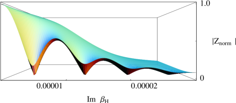
FIG. 5.: $3d$ view of $\left|Z_{\mathrm{norm}}\right|$ near to the first zeroes at $\beta_{G}=12$, $80^{3}$ and $M_{H}^{*}=70$ GeV

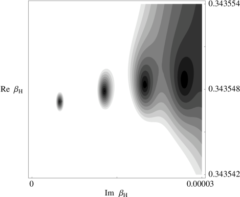
FIG. 6.: Contour plot of $\left|Z_{\mathrm{norm}}\right|$ below 0.2 at $\beta_{G}=12$, $80^{3}$ and $M_{H}^{*}=70$ GeV with height differences of 0.02

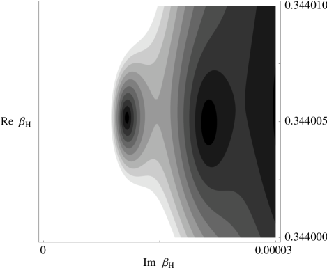
FIG. 7.: Same as Fig. 6 at $\beta_{G}=12$, $80^{3}$ and $M_{H}^{*}=76$ GeV

FIG. 8.: First two zeroes at $\beta_{G}=12$ and $M_{H}^{*}=70$ GeV for different lattice sizes

FIG. 9.: Logarithm of the imaginary part of first zeroes at different $\lambda_{3}/g_{3}^{2}$ vs. logarithm of the physical length $\ln(lg_{3}^{2})$ together with the fit described in the text

FIG. 10.: Fitted distance $R$ as function of $\lambda_{3}/g_{3}^{2}$

FIG. 11.: Fitted power $\nu$ as function of $\lambda_{3}/g_{3}^{2}$

$M_{H}^{*}$	$\beta_{G}$	$L$	$\beta_{H}$	sweeps	$M_{H}^{*}$	$\beta_{G}$	$L$	$\beta_{H}$	sweeps
70	12	30	0.343480	30000	74	12	64	0.343848	20000
70	12	30	0.343540	50000	74	12	64	0.343850	25000
70	12	30	0.343600	40000	74	12	64	0.343852	30000
70	12	40	0.343540	20000	74	12	80	0.3438486	40000
70	12	40	0.343560	20000	74	12	96	0.3438486	40000
70	12	48	0.343440	75000	76	12	30	0.343980	20000
70	12	48	0.343520	40000	76	12	30	0.344000	80000
70	12	48	0.343540	80000	76	12	30	0.344040	20000
70	12	48	0.343544	120000	76	12	40	0.343990	20000
70	12	48	0.343546	20000	76	12	40	0.344000	30000
70	12	48	0.343548	120000	76	12	40	0.344020	20000
70	12	48	0.343560	40000	76	12	48	0.343994	25000
70	12	48	0.343580	110000	76	12	48	0.344000	35000
70	12	64	0.343546	90000	76	12	48	0.344006	35000
70	12	64	0.343548	120000	76	12	48	0.344012	10000
70	12	64	0.343549	20000	76	12	64	0.344000	40000
70	12	64	0.343550	100000	76	12	64	0.344006	40000
70	12	80	0.343546	40000	76	12	80	0.344002	20000
70	16	32	0.340780	40000	76	12	80	0.344002	40000
70	16	32	0.340800	40000	76	12	80	0.344006	25000
70	16	32	0.340820	40000	76	16	32	0.341100	20000
70	16	40	0.340780	40000	76	16	32	0.341120	40000
70	16	40	0.340800	100000	76	16	32	0.341140	20000
70	16	40	0.340820	40000	76	16	40	0.341120	30000
70	16	48	0.340700	45000	76	16	40	0.341124	30000
70	16	48	0.340780	45000	76	16	40	0.341130	20000
70	16	48	0.340800	90000	76	16	48	0.341124	35000
70	16	48	0.340820	45000	76	16	48	0.341128	20000
70	16	64	0.340796	40000	76	16	64	0.341124	40000
70	16	64	0.340800	80000	76	16	64	0.341128	20000
70	16	64	0.340804	40000	76	16	80	0.341126	20000
70	16	80	0.340802	30000	76	16	80	0.341130	30000
74	12	48	0.343850	40000	80	16	80	0.341360	40000

TABLE I.: Statistics

$m_{H}/$GeV	$T_{c}$/GeV	$g^{2}(m_{W})$
67.0(8)	154.8(2.6)	0.423
72.4(9)	110.0(1.5)	0.429

TABLE II.: Some quantities at $\lambda_{3{\mathrm{c}rit}}/g_{3}^{2}=0.102$ ($M_{H\mathrm{crit}}^{*}=72.2$ GeV); upper row without fermions, lower including top

REFERENCES

- [1] F. Karsch, T. Neuhaus, A. Patkós and J. Rank, Nucl. Phys. B(Proc. Suppl.) 53 623 (1997).
-
[2]
K. Kajantie, Nucl. Phys. B(Proc.Suppl.)42 103 (1995);
K. Jansen, Nucl. Phys. B(Proc.Suppl.)47 196 (1996);
K. Rummukainen, Nucl. Phys. B(Proc.Suppl.)53 30 (1997). - [3] B. Bunk, E.-M. Ilgenfritz, J. Kripfganz and A. Schiller, Phys. Lett. B284 371 (1992); Nucl. Phys. B403 112 (1993).
-
[4]
F. Csikor, Z. Fodor, J. Hein and J. Heitger,
Phys. Lett. B357 156 (1995);
Z. Fodor, J. Hein, K. Jansen, A. Jaster and I. Montvay, Nucl. Phys. B439 147 (1995);
F. Csikor, Z. Fodor, J. Hein, A. Jaster and I. Montvay, Nucl. Phys. B474 421 (1996). -
[5]
K. Farakos, K. Kajantie, K. Rummukainen and M. Shaposhnikov,
Nucl. Phys. B425 67 (1994);
K. Kajantie, M. Laine, K. Rummukainen, M. Shaposhnikov, Nucl. Phys. B458 90 (1996). - [6] K. Kajantie, M. Laine, K. Rummukainen and M. Shaposhnikov, Nucl. Phys. B466 189 (1996).
- [7] E.-M. Ilgenfritz, J. Kripfganz, H. Perlt and A. Schiller, Phys. Lett. B356 561 (1995).
- [8] M. Gürtler, E.-M. Ilgenfritz, J. Kripfganz, H. Perlt and A. Schiller, Nucl. Phys. B483 383 (1997).
- [9] K. Kajantie, M. Laine, K. Rummukainen and M. Shaposhnikov, Nucl. Phys. B493 413 (1997).
- [10] M. Reuter and C. Wetterich, Nucl. Phys. B408 91 (1993).
- [11] B. Bergerhoff and C. Wetterich, hep-ph/9508352, hep-ph/9611462.
- [12] N. Tetradis, Nucl. Phys. B488 92 (1997).
- [13] W. Buchmüller and O. Philipsen, Nucl. Phys. B443 47 (1995).
- [14] K. Kajantie, M. Laine, K. Rummukainen and M. Shaposhnikov, Phys. Rev. Lett. 77 2887 (1996).
-
[15]
C. N. Yang, T. D. Lee,
Phys. Rev. 87 404, 410 (1952);
K. Huang, Statistical Mechanics, John Wiley and Sons, New York 1987;
M. E. Fisher, in: Lectures in theoretical physics, vol. 7C, University of Colorado Press, 1965. - [16] E. Marinari, Optimized Monte Carlo Methods, Lectures at the 1996 Budapest Summer School on Monte Carlo Methods, preprint cond-mat/9612010.
- [17] Y. Aoki, Nucl. Phys. B(Proc. Suppl.)53 609 (1997) and hep-lat/9612023.
- [18] A. Ferrenberg, R. Swendsen, Phys. Rev. Lett. 61 2635 (1988); 63 1195 (1989).
-
[19]
C. Borgs and R. Kotecký,
J. Stat. Phys. 61 79 (1990);
C. Borgs, R. Kotecký and S. Miracle-Solé, J. Stat. Phys. 62 529 (1991). - [20] G. D. Moore, Nucl. Phys. B493 439 (1997).
- [21] B. Bunk, Nucl. Phys. B(Proc. Suppl.) 42 566 (1995).
- [22] M. Laine, Phys. Lett. B385 249 (1996).
- [23] M. Gürtler, E.-M. Ilgenfritz and A. Schiller, Z. Phys. C to appear, hep-lat/9702020.