21 April 1997 JINR E2-97-142
FSU-SCRI-97-37
IFUP–TH 14/97

We study the heavy charge potential in the Coulomb phase of pure gauge compact $U(1)$ theory on the lattice. We calculate the static potential $V_{W}(T,{\vec{R}})$ from Wilson loops on a $16^{3}\times 32$ lattice and compare with the predictions of lattice perturbation theory. We investigate finite size effects and, in particular, the importance of non–Coulomb contributions to the potential. We also comment on the existence of a maximal coupling in the Coulomb phase of pure gauge $U(1)$ theory.

1 Introduction

In 1974 Wilson proposed the compact lattice formulation of pure gauge $U(1)$ theory [2]. The action of this model is

$$S_{W}(U)=\beta\sum_{x}\sum_{\mu>\nu}\Bigl{(}1-\cos\theta_{x,\mu\nu}\Bigr{)}~{},\qquad\beta=\frac{1}{g^{2}}~{},$$ (1)

where $~{}g^{2}~{}$ is the bare coupling constant, and the link variables are $U_{x\mu}=\exp(i\theta_{x\mu})$, $\theta_{x\mu}\in(-\pi,\pi]$. The plaquette angles are given by $\theta_{x,\,\mu\nu}=\theta_{x,\,\mu}+\theta_{x+\hat{\mu},\,\nu}-\theta_{x+\hat{\nu},\,\mu}-\theta_{x,\,\nu}$. This action makes up the pure gauge part of the full QED action $S_{QED}$, which is supposed to be compact if we consider QED as arising from a subgroup of a non–abelian (e.g., grand unified) gauge theory [3].

The average of any gauge–invariant functional ${\cal O}(U)$ is

$$\langle{\cal O}(U)\rangle=Z^{-1}\int\!\prod_{x\mu}\!dU_{x\mu}\,{\cal O}(U)\cdot e^{-S_{W}(U)}~{},\qquad dU_{x\mu}=\frac{d\theta_{x\mu}}{2\pi}~{},$$ (2)

where $Z$ is the partition function, defined formally by $\langle 1\rangle=1$. At small enough $~{}\beta$’s the strong coupling expansion shows an area–law behaviour of the Wilson loops, while at large $~{}\beta$’s a deconfined phase exists. The two phases are separated by a phase transition at some ‘critical’ value $\beta^{\ast}$ whose existence was assumed in [2]. The weak coupling – deconfined – phase is expected to be a Coulomb phase, i.e., a phase with massless noninteracting vector bosons (photons) and Coulomb–like interactions between static charges.

There are scarcely any doubts about the existence of the Coulomb phase in the weak coupling region for Wilson’s QED, though – to our knowledge – there is no rigorous proof. It is worthwhile to mention that for the Villain approximation [4] such a proof is available [5, 6]. However, a detailed study has shown that the Villain action is quantitatively a rather bad approximation to the Wilson action in the weak coupling region [7].

A perturbative expansion suggests for the lattice potential $V^{latt}({\vec{R}})$ the expression

$$V^{latt}({\vec{R}})=\sum_{n=1}^{\infty}g^{2n}\cdot V_{n}({\vec{R}})~{},$$ (3)

where up to an additive constant $~{}V_{1}~{}$ is the lattice analog of the

continuum Coulomb potential $~{}\sim 1/4\pi R~{}$ (for an explicit expression see (9) below). One–loop corrections ($\sim g^{4}$) do not change the functional dependence of the potential but at the two–loop level ($\sim g^{6}$) non–Coulomb–like contributions appear (see below). The analytical and numerical study of these contributions, as well as of the finite volume behavior of the potential, constitutes the aim of the present work.

The behavior of the heavy charge potential in the weak coupling phase in pure $U(1)$ gauge theory was the subject of several numerical studies (see, e.g. [8, 9, 10, 11]). In all cases consistency with a Coulomb–like behavior was reported. However, we feel that a more elaborate and systematic study is necessary. In particular, Monte Carlo simulations give precise enough measurements of the potential, that finite size effects and finite lattice spacing effects, i.e., deviations of the lattice Coulomb potential from the continuum $1/R$ behavior should not be neglected. In addition, finite $T$ effects in the extraction of the potential from Wilson loops have to be taken into account. We shall find, on the other hand, that the non-Coulomb–like contributions to the potential are negligible.

We consider this systematic study of the Coulomb phase in pure gauge $U(1)$ theory a necessary step before attempting an investigation of lattice QED with fermions with the aim of obtaining a continuum limit that reproduces weak coupling continuum QED.

The second section is devoted to the two-loop perturbative study of the potential, $V_{P}({\vec{R}})$, as extracted from Polyakov loop correlations. Special emphasis has been put on the study of the non–Coulomb–like contributions that appear at two–loop order, i.e., at order $O(g^{6})$. In the third section we discuss the potential, $V_{W}(T,{\vec{R}})$, as extracted from Wilson loops. We present the results of Monte Carlo simulations and their comparison with perturbation theory. Indeed, perturbation theory will play a major role in our extraction of a renormalized coupling, $g_{R}^{2}$, from the numerical simulations. In section 4 we address the question of the existence of a maximal coupling in pure gauge U(1). The last section is reserved for conclusions and discussions.

2 The potential from Polyakov loop correlations at $O(g^{6})$

One way to define the heavy charge potential $V=V_{P}({\vec{R}})$ is

$$V_{P}({\vec{R}})=-\frac{1}{N_{4}}\cdot\ln\Gamma_{P}({\vec{R}})~{},$$ (4)

where we consider a finite lattice of size $N_{s}^{3}\times N_{4}$ and $\Gamma_{P}({\vec{R}})$ is the Polyakov loop correlator

$$\Gamma_{P}({\vec{R}})=\frac{1}{Z}\int_{A}~{}e^{ig\sum_{x\mu}J^{P}_{x\mu}A_{x\mu}}\cdot e^{-S_{W}(A)}~{},$$ (5)

if the currents $J^{P}_{x\mu}$ correspond to a static heavy charge–anticharge pair

$$J^{P}_{4}(x) = \left\{\begin{array}[]{ll}\delta_{{\vec{x}},{\vec{0}}}-\delta_{{\vec{x}},{\vec{R}}}&\quad\mbox{at}\quad 0\leq x_{4}\leq N_{4}-1\\ 0&\quad\mbox{otherwise}\end{array}\right.~{},$$ (8)

and $J^{P}_{i}(x)=0$, $i=1,2,3$.

We calculated the potential $V_{P}({\vec{R}})$ perturbatively up to order $O(g^{6})$. Graphically the different contributions are shown in Figure 1.

Figure 1: Different diagrams contributing to the potential $V_{P}({\vec{R}})$.

In the tree approximation (Figure 1a) one obtains the lattice Coulomb potential

$$g^{2}V_{Coul}^{(N_{s})}({\vec{R}})=\frac{g^{2}}{N_{s}^{3}}\sum_{{\vec{p}}\neq 0}\frac{1-\cos{\vec{p}}{\vec{R}}}{{\vec{\cal K}}^{\,2}}~{},$$ (9)

where ${\cal K}_{i}=2\sin\frac{p_{i}}{2}$. In the infinite volume limit, $~{}N_{s}\to\infty~{}$, this potential becomes

$$g^{2}V_{Coul}^{(\infty)}({\vec{R}})=\frac{g^{2}}{(2\pi)^{3}}\int_{-\pi}^{\pi}\!d{\vec{p}}~{}\frac{1-\cos{\vec{p}}{\vec{R}}}{{\vec{\cal K}}^{\,2}}~{},\quad N_{s}\longrightarrow\infty~{},$$ (10)

The continuum analog of this expression is

$$g^{2}V_{cont}({\vec{R}})=-\frac{g^{2}}{4\pi R}+\mbox{Const}~{}.$$ (11)

The lattice Coulomb potential defined in eq. (9) becomes close to the continuum expression in eq. (11) when $1\ll R\ll\frac{1}{2}N_{s}~{}$ for sufficiently large lattice size $N_{s}$. For lattice sizes that are typically used in numerical simulations (i.e. $N_{s}\sim 16\div 32$) the lattice Coulomb potential in eq. (9) differs considerably from the continuum expression in eq. (11).

The $O(g^{4})$ contribution (Figure 1b) as well as $O(g^{6})$ contributions shown in Figures 1c to 1e result in a renormalization of the coupling without changing the form of the potential. However, two diagrams at order $\sim O(g^{6})$ contain non–Coulomb–like contributions. One of them is the four–prong–spider graph (Figure 1f) which gives the contribution to the potential

$$V^{(f)}({\vec{R}}) = -\frac{2g^{6}}{3N_{s}^{9}}\sum_{\{{\vec{p}}^{(i)}\}}\delta_{{\vec{p}}^{(1)}+\ldots+{\vec{p}}^{(4)},0}\prod_{i=1}^{4}\sin\frac{{\vec{p}}^{(i)}{\vec{R}}}{2}\cdot\sum_{j=1}^{3}\prod_{i=1}^{4}\frac{{\cal K}_{j}(p^{(i)})}{{\vec{\cal K}}^{2}(p^{(i)})}~{}.$$ (12)

Another non–Coulomb–like contribution comes from the two–loop bubble diagram shown in Figure 1g

$$V^{(g)}({\vec{R}}) = \frac{g^{6}}{48}V_{Coul}({\vec{R}})+V^{(g)}_{nCoul}({\vec{R}})~{},$$ (13)

$$V^{(g)}_{nCoul}({\vec{R}}) = \frac{g^{6}}{6N_{s}^{3}}\sum_{{\vec{p}}}\frac{1-\cos{\vec{p}}{\vec{R}}}{({\vec{\cal K}}^{\,2})^{2}}\sum_{i,j=1}^{3}{\cal K}_{i}{\cal K}_{j}\cdot\Bigl{(}T_{ij}({\vec{p}})-T_{ij}({\vec{0}})\Bigr{)}~{},$$ (14)

where

$$T_{ij}({\vec{p}})=\frac{1}{(N_{4}N_{s}^{3})^{2}}\sum_{qq^{\prime}}D_{ij}(q)D_{ij}(q^{\prime})D_{ij}(p-q-q^{\prime})~{},\quad D_{ij}(q)=\frac{{\cal K}_{i}{\cal K}_{j}+{\cal K}_{4}^{2}\cdot\delta_{ij}}{{\cal K}^{2}}(q)~{}.$$ (15)

Therefore, up to order $O(g^{6})$ the static charge potential $V_{P}({\vec{R}})$ is

$$V_{P}({\vec{R}})=g^{2}_{2-loop}\cdot V_{Coul}({\vec{R}})+g^{6}\cdot V_{nCoul}({\vec{R}})~{},$$ (16)

with

$$V_{nCoul}({\vec{R}})=V^{(f)}({\vec{R}})+V^{(g)}_{nCoul}({\vec{R}})~{},$$ (17)

and where

$$g^{2}_{2-loop}=g^{2}(1+\frac{1}{4}g^{2}+\frac{11}{96}g^{4})~{}.$$ (18)

To get an idea of the possible importance of the non–Coulomb term, we computed it by numerically performing the necessary lattice momentum sums on several lattices up to size $16^{4}$. As an example we compare $V_{nCoul}$ with $V_{Coul}$ in Figure 2. We see that $V_{nCoul}$ is almost three orders of magnitude smaller than $V_{Coul}$, a difference that will even be enhanced when including the coupling constants for weak coupling. Furthermore $V_{nCoul}$ approaches its asymptotic value much faster than $1/R$. Since the long distance behavior is governed by the small momentum region, we can estimate it in the infinite volume limit from power counting in the small momentum region of the integrals. For the two-loop bubble diagram, eq. (14), since the zero-momentum part corresponding to $T_{ij}({\vec{0}})$, which contributes to $V_{Coul}$, was split off, we expect a $1/R^{3}$ approach to a constant. For the four–prong–spider graph, eq. (12), we expect, apart from a constant, a $1/R^{5}$ fall-off at large distance. Log–log plots of the numerically computed non-Coulomb contributions on finite lattices confirm these expectations.

Figure 2: Comparison of the non–Coulomb part $V_{nCoul}$, eq. (17), of the potential to the (lattice) Coulomb part $V_{Coul}$, eq. (9), on a $16^{4}$ lattice.

From the large distance behavior in the infinite volume limit we can also estimate the finite size effects. Periodic boundary conditions can be mimicked by mirror charges, e.g. for an on-axis distance the infinite volume $1/R^{n}$ becomes in a finite volume with box size $N_{s}$,

$$\frac{1}{R^{n}}+\frac{1}{(N_{s}-R)^{n}}=\frac{1}{R^{n}}+\frac{1}{N_{s}^{n}}+n\frac{R}{N_{s}^{n+1}}+\frac{1}{N_{s}^{n}}O\left(\frac{r^{2}}{N_{s}^{2}}\right)$$ (19)

Therefore we expect the leading finite volume corrections to affect the constant at $O(1/N_{s})$ for $V_{Coul}$ and only at $O(1/N_{s}^{3})$ for $V_{nCoul}$. The finite size effects in $V_{nCoul}$ appear to be much smaller than those in $V_{Coul}$. Our numerical results are in agreement with this expectation.

3 The potential and the renormalized coupling from Wilson loops

The potential can also be obtained from Wilson loops: $V=V_{W}(T,{\vec{R}})$. It is defined as follows

$$V_{W}(T;{\vec{R}})=\ln\frac{W(T,{\vec{R}})}{W(T+1,{\vec{R}})}~{},$$ (20)

where $~{}W(T,{\vec{R}})~{}$ is the Wilson loop with ‘time’ extension $T$ and space extension ${\vec{R}}$.

The Wilson loop can be on–axis or off-axis, and the space–like parts of the loop can include the contribution of many different contours. In our calculations we have chosen planar loops and two types of non–planar contours: the ‘plane-diagonal’ contour with space–like part in the plane $(x_{2},x_{3})$ at fixed $x_{1}$ (say, $x_{1}=0$) connecting points $x_{2}=x_{3}=0$ and $x_{2}=x_{3}=R_{0}$, and the ‘space-diagonal’ contour in the $3d$ space $(x_{1},x_{2},x_{3})$ connecting points $x_{1}=x_{2}=x_{3}=0$ and $x_{1}=x_{2}=x_{3}=R_{0}$. For the off-axis loops we average over all paths that follow the straight line between the endpoints as closely as possible. For example, for the loop through the origin and $x_{2}=x_{3}=R_{0}$ the paths considered go through all points with $x_{2}=x_{3}$ in between. We average over all combinations of first taking a step in the 2-direction followed by a step in the 3-direction and vice versa.

At lowest order in perturbation theory the potential $V_{W}(T;{\vec{R}})$ becomes

$$V_{W}(T;{\vec{R}})=w(T,{\vec{R}})-w(T+1,{\vec{R}})~{},$$ (21)

with $w(T,{\vec{R}})$ the $O(g^{2})$ part of the Wilson loop, which in turn, in Feynman gauge, can be split as

$$w(T,{\vec{R}})=w_{s}(T,{\vec{R}})+w_{t}(T,{\vec{R}})~{},$$ (22)

where $~{}w_{t}~{}$ and $~{}w_{s}~{}$ are contribution of the time–time (‘electric’) and space–space (‘magnetic’) parts, respectively. The time–time contribution is

$$w_{t}(T,{\vec{R}})=-\frac{g^{2}}{N_{4}N_{s}^{3}}\sum_{p}(1-\cos{\vec{p}}{\vec{R}})\cdot\frac{1-\cos p_{4}T}{1-\cos p_{4}}\cdot G_{0}(p)~{},$$ (23)

where $G_{0}(p)=1/{\cal K}^{2}$. It is easy to show that in the limit $~{}N_{4}\rightarrow\infty~{},~{}~{}T\rightarrow\infty~{},~{}~{}T\ll N_{4}~{}$ the ’time’–like (’electric’) part of the potential gives the lattice Coulomb potential as obtained from Polyakov loop correlations and given in eq. (9).

For the planar Wilson loops in the plane $~{}(x_{3},x_{4})~{}$ the space–space contribution $~{}w_{s}~{}$ is

$$w_{s}=-\frac{g^{2}}{N_{4}N_{s}^{3}}\sum_{p\neq 0}(1-\cos p_{4}T)\cdot\frac{1-\cos p_{3}R}{1-\cos p_{3}}\cdot G_{0}(p)~{}.$$ (24)

For the ‘plane-diagonal’ contour, in the plane $~{}(x_{2},x_{3})~{}$ at fixed $~{}x_{1}~{}$ connecting points $~{}x_{2}=x_{3}=0~{}$ with $~{}x_{2}=x_{3}=R_{0}~{}$ the space–space contribution is

$$w_{s}=-\frac{g^{2}}{2N_{4}N_{s}^{3}}\sum_{p\neq 0}(2+\cos p_{2}+\cos p_{3})\cdot\frac{1-\cos R_{0}(p_{2}+p_{3})}{1-\cos(p_{2}+p_{3})}\cdot(1-\cos p_{4}T)\cdot G_{0}(p)~{},$$ (25)

and finally for the ‘space-diagonal’ contour connecting points $~{}x_{1}=x_{2}=x_{3}=0~{}$ with $~{}x_{1}=x_{2}=x_{3}=R_{0}~{}$ the space–space contribution is

$$w_{s} = \frac{2g^{2}}{N_{4}N_{s}^{3}}\sum_{p\neq 0}{\cal A}({\vec{p}})\cdot\frac{1-\cos R_{0}(p_{1}+p_{2}+p_{3})}{1-\cos(p_{1}+p_{2}+p_{3})}\cdot(1-\cos p_{4}T)\cdot G_{0}(p)~{},$$

$${\cal A} = -\frac{1}{18}\left[~{}2\cos\frac{p_{2}+p_{3}}{2}+\cos\frac{p_{2}-p_{3}}{2}~{}\right]^{2}+\Bigl{\{}\mbox{permutations of}~{}p_{1},p_{2},p_{3}\Bigr{\}}~{}.$$ (26)

The contribution from $w_{s}$ to $V_{W}(T;{\vec{R}})$ vanishes in the limit $T\to\infty$ and in this limit the potentials extracted from Polyakov line correlations and from Wilson loops agree. At finite $T$, however, $w_{s}$ gives a contribution $\approx cR/T^{2}$ to $V_{W}(T;{\vec{R}})$. At a finite $T$ the potential $V_{W}(T;{\vec{R}})$ hence appears to have a small confining contribution. $V_{W}(T;{\vec{R}})$ therefore needs to be either carefully extrapolated to infinite $T$, or the finite $T$ effect has to be taken into account in the analysis, as we shall do in this paper.

Just as was the case for the potential obtained from Polyakov loop correlations, at one–loop level the only effect is a renormalization of the coupling $g^{2}\to g^{2}(1+\frac{1}{4}g^{2})$. At two loops in the perturbative expansion we only considered, for simplicity, planar Wilson loops. We find the same structure as for the potential from Polyakov loops, eq.s (16) and (17). In particular, the two–loop renormalization of the coupling is identical, as given in eq. (18).

Our Monte Carlo data were produced on a $~{}16^{3}\times 32~{}$ lattice for $11$ values of $~{}\beta~{}$ shown in Table  1. We measured planar and nonplanar Wilson loops $~{}W(T,{\vec{R}})~{}$ with $~{}T\leq T_{max}=15~{}$ and $~{}R\leq R_{max}=8\sqrt{3}$. To decrease the statistical noise we have used the Parisi–Petronzio–Rapuano trick [12] for all time–like links. Because of this we do not have a valid measurement of the potential at distance $R=1$, and this distance is therefore excluded from all further considerations.

In the Coulomb phase the potential obtained from Monte Carlo simulations is expected to be very similar to the perturbative lattice Coulomb potential. Since the latter can have sizable finite size and finite $T$ effects, as discussed earlier, we decided to use as a fit formula for the numerical potential $V_{W}(T;{\vec{R}})$ the lowest order perturbative expression defined in eq.’s (21) to (26), with the only fit parameter being the renormalized coupling constant $g^{2}_{R}$. The success of such fits will indicate that the non-Coulomb contributions are small, like in perturbation theory, and that non-perturbative effects just go into the renormalization of the coupling. The number of degrees of freedom, $N_{d.o.f.}$ in our fits varied between $N^{max}_{d.o.f.}=344$ and $N^{min}_{d.o.f.}=31$ with decreasing $\beta$, from $\beta=10$ to $\beta=1.015$. In all the cases we obtained $\chi^{2}/N_{d.o.f.}\mbox{}_{\textstyle\sim}^{\textstyle<}1.0$ (with the only exception being for $\beta=1.015$ where $\chi^{2}/N_{d.o.f.}\simeq 2.1$). As an example we show in Figure 3 the $R$–dependence of the potential $V_{W}(T;{\vec{R}})$ at $T=1$ and $T=15$ (circles). Crosses show the corresponding values of $g^{2}_{R}V_{Coul}(T;{\vec{R}})$ with the fitted $g^{2}_{R}$. We would like to emphasize that, even at $T=15$, the potential from nonplanar Wilson loops cannot be fitted with a continuum–like $1/R$ ansatz, which can be attempted when only planar Wilson loops are available (see e.g. [10, 11]).

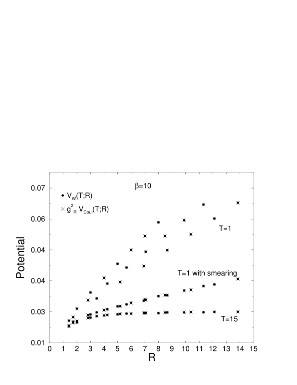
Figure 3: The Wilson loop potential $V_{W}(T;{\vec{R}})$ (circles) and the corresponding perturbative potential $g^{2}_{R}V_{Coul}(T;{\vec{R}})$ (crosses) at $\beta=10$ on a $16^{3}\times 32$ lattice with and without smearing. For $T=15$ the potential from smeared and normal Wilson loops would be indistinguishable in the figure.

At large values of $\beta$ ($\beta\geq 5$) our one-parameter fit works well for the whole set of data points, i.e. all points with $1\leq T\leq 15$ and $1<R\leq 8\sqrt{3}$ ($N_{d.o.f.}=344$). The non–Coulomb–like corrections are therefore negligible despite our rather small statistical errors. With decreasing $\beta$ these corrections become noticeable at small values of $R$ (recall the fast fall-off of $V_{nCoul}$ like $1/R^{3}$) and small values of $T$. After excluding the data points corresponding to these small $R$ and $T$ values from the fit, we obtained fits with a high confidence level, but fewer degrees of freedom, as described above. Remarkably, the lattice Coulomb potential works, at least at large distance, really well even at $\beta$–values very close to the phase transition point, $\beta^{\ast}$, to the confined phase. This observation in fact constitutes one of the main results of this paper.

The extracted values of the renormalized coupling $g^{2}_{R}$ as well as the perturbative values $g^{2}_{1-loop}$ and $g^{2}_{2-loop}$ are listed in Table 1 and shown in Figure 4. The difference between $g^{2}_{R}$ and the perturbative value $g^{2}_{2-loop}$ becomes noticeable at $\beta\mbox{}_{\textstyle\sim}^{\textstyle<}2.0$. This is the region where one expects the perturbative three–loop contributions to become important. In addition nonperturbative effects may start to significantly contribute.

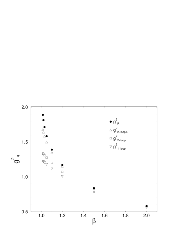
Figure 4: The renormalized coupling $g^{2}_{R}$ extracted from the fit on a $16^{3}\times 32$ lattice as compared with $1$–loop and $2$–loop perturbative values.

$\beta$	$g^{2}_{1-loop}$	$g^{2}_{2-loop}$	$g^{2}_{R}$
1.015	1.22789	1.33747	1.892(5)
1.020	1.22068	1.32866	1.815(5)
1.030	1.20652	1.31138	1.716(4)
1.050	1.17914	1.27812	1.585(2)
1.100	1.11570	1.20179	1.3913(10)
1.200	1.00694	1.07325	1.1707(7)
1.500	0.77778	0.81173	0.8379(5)
2.000	0.56250	0.57682	0.5833(3)
5.000	0.21000	0.21092	0.21104(4)
7.000	0.14796	0.14829	0.14834(3)
10.00	0.10250	0.10262	0.10263(3)

Table 1: The renormalized coupling $g^{2}_{R}$ extracted from the fit on a $32\times 16^{3}$ lattice as compared with $1$–loop and $2$–loop perturbative values.

In numerical simulations of QCD it has become standard to use a smearing procedure to improve the signal–to–noise ratio. In the computation of Wilson loops the space–like link elements $U_{k}$ are replaced be recursively computed “smeared links” $U^{(n)}_{k}$

$$U^{(n+1)}_{xk}=P\Bigl{[}\alpha U^{(n)}_{xk}+\sum_{j\neq k}\bigl{(}U^{(n)}_{xj}U^{(n)}_{x+j,k}U^{(n)\dagger}_{x+k,j}+U^{(n)\dagger}_{x-j,j}U^{(n)}_{x-j,k}U^{(n)}_{x-j+k,j}\bigr{)}\Bigr{]},\quad j,k=1,2,3~{},$$ (27)

where $P$ indicates a projection onto the gauge group. The choice of $\alpha$, the weight of the direct link relative to the “staples”, and the number of smearing iterations $n_{sme}$ are parameters that can be optimized.

At lowest perturbative order the recursive relation eq. (27) becomes for Fourier transformed fields

$$A^{(n+1)}_{k}(p)=\frac{1}{\alpha+4}\Bigl{[}A^{(n)}_{k}(p)\bigl{(}\alpha+\sum_{j\neq k}2\cos p_{j}\bigr{)}+4\sin\frac{p_{k}}{2}\sum_{j\neq k}A^{(n)}_{j}(p)\sin\frac{p_{j}}{2}\Bigr{]}.$$ (28)

This relation can easily be iterated and inserted in the numerical computation of the momentum sums to obtain the lowest order perturbative contribution to the potential from the space–space parts of the Wilson loops.

In Figure 3 we show the effect of smearing on the potential extracted at $T=1$ (circles) for $\beta=10$. The parameters of smearing were chosen as $\alpha=4$ and $n_{sme}=6$. The crosses on the top of these circles indicate the values of the potential obtained from the one-parameter fit to the perturbative form, as described above. In this case the $\chi^{2}$–value is somewhat larger ($\chi^{2}/N_{d.o.f.}\sim 2.9$). However the extracted value of the renormalized coupling $g^{2}_{R}$ appears to be very stable with respect to the smearing procedure, and $g^{2}_{R}$ from the smeared loops coincides (within errorbars) with the coupling found without smearing.

For non–abelian lattice gauge theory it has proved useful, in perturbative computations, to use an the ‘improved’ coupling, such as $g^{2}_{E}$ [15, 16]

$$g^{2}_{E}\equiv\frac{1}{c_{1}}\Bigl{(}1-\langle U_{p}\rangle\Bigr{)}~{},$$ (29)

where $U_{p}$ denotes the plaquette and $c_{1}=1/4$ is the first coefficient in its perturbative expansion. For pure gauge $U(1)$ the perturbative expansion of $\langle U_{p}\rangle$ is known to three loops[17]

$$\langle U_{p}\rangle=1-\frac{1}{4}g^{2}-\frac{1}{32}g^{4}-0.0131185g^{6}-0.00752g^{8}+\ldots~{}.$$ (30)

From this we get a perturbative expansion of $g^{2}_{E}$ in terms of the bare $g^{2}$. We then can express $g^{2}$ in terms of $g^{2}_{E}$ and substitute in the perturbative formula for $g^{2}_{2-loop}$, eq. (18),

$$g^{2}_{2-loop,E}=g^{2}_{E}(1+\frac{1}{8}g^{2}_{E}+0.0308594g^{4}_{E}+\ldots).$$ (31)

The plaquette averages, $g^{2}_{E}$ and the corresponding prediction for $g^{2}_{2-loop,E}$ from eq. (31) is listed in Table 2. Comparing with Table 1 we see, that $g^{2}_{2-loop,E}$ based on the ‘improved’ coupling $g^{2}_{E}$ is indeed a somewhat better prediction for $g^{2}_{R}$ than the purely perturbative $g^{2}_{2-loop}$. This fact can also be seen in Figure 4.

$\beta$	$\langle U_{p}\rangle$	$g^{2}_{E}$	$g^{2}_{2-loop,E}$
1.015	0.66147(2)	1.3541	1.6800
1.02	0.66749(3)	1.3301	1.6429
1.03	0.67680(2)	1.2928	1.5859
1.05	0.69104(2)	1.2358	1.5002
1.1	0.71674(2)	1.1330	1.3501
1.2	0.751625(10)	0.9935	1.1551
1.5	0.812599(6)	0.7496	0.8363
2	0.864810(8)	0.5408	0.5835
5	0.9486330(24)	0.20547	0.21109
7	0.9636091(13)	0.14556	0.14833
10	0.9746754(8)	0.10130	0.10262

Table 2: The average plaquette, $\langle U_{p}\rangle$, the extracted $g^{2}_{E}$ and the corresponding prediction for $g^{2}_{2-loop,E}$ from eq. (31)

4 Universal maximal coupling?

In paper [13] the existence of a universal finite value $4\pi\alpha_{c}\equiv g^{2}_{c}$ was predicted at the deconfinement point, $\beta^{\ast}$, based on an analogy with the $2d$ Kosterlitz–Thouless transition. The mechanism of the transition in the pure gauge $U(1)$ theory and in the $2d$ $XY$ model was shown to be the termination of the massless phase by a topological disordering. The approach to this maximum finite coupling was conjectured as

$$g^{2}_{R}=g^{2}_{c}-c\left(\beta-\beta^{\ast}\right)^{\lambda}$$ (32)

with the estimates $g^{2}_{c}=4\pi\alpha_{c}=1.90\pm 0.10$ and $\lambda=0.5(1)$ [14].

We have attempted fits of the form eq. (32) to our data. A four–parameter fit to the 5 data points with the smallest $\beta$ gives $\beta^{\ast}=1.007(3)$, $g^{2}_{c}=2.4(3)$ and $\lambda=0.27(8)$ with a $\chi^{2}=0.15$ for 1 degree of freedom. Including more data points decreases the estimate of $\beta^{\ast}$ and increases the estimate of $g^{2}_{c}$. The above estimate for $\beta^{\ast}$ is somewhat smaller then the value $\beta^{\ast}=1.011(2)$ found in [10]. Constraining $\beta^{\ast}$ to 1.011 a three–parameter fit gives now $g^{2}_{c}=2.12(2)$ and $\lambda=0.38(2)$ with a $\chi^{2}=1.20$ for 2 degrees of freedom, or, using only 4 data points, $g^{2}_{c}=2.08(4)$ and $\lambda=0.43(5)$ with a $\chi^{2}=0.01$ for 1 degree of freedom. Varying $\beta^{\ast}$ from 1.009 to 1.013 gives variations somewhat larger than the statistical errors. Our final estimates are then

$$g^{2}_{c}=2.08\pm 0.14~{}~{}~{}~{}~{}~{}~{}{\rm and}~{}~{}~{}~{}~{}~{}~{}\lambda=0.43\pm 0.10$$ (33)

with the errors dominated by systematic uncertainties. Obviously, more data points in the “critical” region would be desirable to make the systematic errors smaller.

The existence of $g^{2}_{c}$ as maximal coupling depends on the presence of the monopole induced phase transition to a confining phase. When the monopoles are suppressed, this phase transition disappears. This leads to the question of whether in that case larger renormalized couplings can be achieved than the above $g^{2}_{c}$. This seems indeed the case as found in [18] in the context of the U(1) Higgs model with suppressed monopoles. We have repeated the measurements of the renormalized coupling for pure U(1) with completely suppressed monopoles on an $8^{3}\times 16$ lattice. The results are listed in Table 3. $g^{2}_{R}$ was extracted exactly as for the model with standard Wilson action described in the previous section. Since our analysis carefully includes finite size (and finite $T$) effects, a lattice of size $8^{3}\times 16$ is sufficient for our purposes here. In Table 3 we list, for comparison, also renormalized couplings for the standard model obtained from an $8^{3}\times 16$ lattice. Comparison with Table 1 shows that the residual finite size effects are indeed very small, even close to the phase transition.

$\beta$	$g^{2}_{R}$(NoMo)	$g^{2}_{R}$(stand)
0.0001	5.19(4)
0.25	3.97(2)
0.5	2.911(11)
1.0	1.445(5)
1.015		1.86(3)
1.02	1.406(3)	1.79(3)
1.05	1.349(3)	1.579(8)
1.2	1.125(2)	1.172(2)
1.5	0.8315(8)	0.8362(13)
2.0	0.5824(5)	0.5831(2)

Table 3: The coupling $g^{2}_{R}$ from an $8^{3}\times 16$ lattice for the standard U(1) model, and for the model with complete monopole suppression.

From Table 3 we see that at larger $\beta$ ($\beta\geq 2.0$) monopole suppression has no effect, as expected, since monopoles are very much suppressed in the standard U(1) model there. For smaller $\beta$, due to the effect from monopoles, $g^{2}_{R}$ raises faster for the standard U(1) model until reaching its maximal value $g^{2}_{c}$ at the phase transition point. With monopoles completely suppressed, $g^{2}_{R}$ raises more slowly. However, the absence of the confinement phase transition, allows $g^{2}_{R}$ to keep growing and to become larger than $g^{2}_{c}$. Although the model with complete suppression of monopole has no phase transition even at $\beta=0$, we stopped our measurements at a small positive value to ensure that the bare coupling remains real.

The maximal coupling $g^{2}_{c}$, however, should be universal for U(1) actions with a monopole induced phase transition, for example the Villain model. The renormalized coupling was measured for the Villain model in [9], albeit only on a $6^{3}\times 4$ lattice. We simulated an $8^{3}\times 16$ lattice and extracted $g^{2}_{R}$ the same way as for the Wilson action. Our results are listed in Table 4.

$\beta$	$g^{2}_{R}$
0.645	2.027(30)
0.65	1.915(24)
0.655	1.868(12)
0.66	1.816(9)
0.67	1.732(6)
0.68	1.672(5)
0.7	1.575(6)
0.75	1.402(2)
0.8	1.285(2)
1.0	1.003(2)

Table 4: The coupling $g^{2}_{R}$ from an $8^{3}\times 16$ lattice for the U(1) model with Villain action.

For the Villain action, there is no perturbative renormalization of the bare coupling. All the renormalization comes from the monopoles. Indeed, up to $\beta=1.0$ the renormalized and bare couplings are almost identical. Only then do the monopoles start to have an appreciable influence and $g^{2}_{R}$ becomes larger than the bare coupling and continues to raise until the phase transition to the confined phase is reached. We made a fit of our data to the form eq. (32). The fit works very nicely for $\beta\leq 0.75$. Including all 8 data points gives a $\chi^{2}=1.23$ for 4 degrees of freedom with

$$g^{2}_{c}=2.12(4)~{},~{}~{}~{}\beta^{\ast}=0.6457(8)~{}~{}~{}{\rm and}~{}~{}~{}\lambda=0.43(4)$$ (34)

in nice agreement with the results for the Wilson action, eq. (33) and confirming the universality of $g^{2}_{c}$. The result eq. (34) is stable when omitting data points from the fits.

5 Conclusions

We have made an analytical and numerical study of compact lattice pure gauge $~{}U(1)~{}$ theory in the Coulomb phase. The main point of interest was the study of the non–Coulomb contributions to the heavy charge potential. For this purpose we calculated perturbatively the heavy charge potential $~{}V_{P}({\vec{R}})~{}$ defined from the Polyakov loop correlations in the 2–loop (i.e., $\sim g^{6}$) approximation. This calculation shows that the non–Coulomb contribution $~{}V_{P}^{nCoul}({\vec{R}})~{}$ is much smaller than the Coulomb contribution $~{}V_{P}^{Coul}({\vec{R}})~{}$, at least at large distances.

The conclusions obtained within perturbation theory were confirmed by numerical calculations of the potential $~{}V_{W}(T;{\vec{R}})~{}$ defined from planar and nonplanar time–like Wilson loops. We used as a fit formula for $~{}V_{W}(T;{\vec{R}})~{}$ the lowest order perturbative expression with the only fit parameter being the renormalized coupling constant $~{}g^{2}_{R}$. These fits worked well for all distances at large $\beta$, and for sufficiently big $~{}T~{}$ and $~{}R$ even down to very close to the phase transition to the strong coupling confined phase. It is worth noting that it is impossible to obtain a good $~{}\chi^{2}~{}$ using for the fit a continuum potential $~{}\sim 1/R$. The values of the renormalized coupling $~{}g^{2}_{R}~{}$ are stable with respect to a smearing procedure.

We confirmed, with better accuracy, the conjectured existence of a universal maximal coupling for $U(1)$ models with a monopole induced confining phase transition. In the model with complete suppression of monopoles, however, even larger renormalized couplings can be reached.

Our main conclusion is that compact pure gauge $U(1)$ theory can serve equally well as a non–compact version to describe the physics of free photons in the weak coupling region. The only difference is a finite, $R$–independent renormalization of the coupling constant $~{}g^{2}\to g^{2}_{R}$ in the compact theory.

References

- [1]
- [2] K. Wilson, Phys. Rev. D10 (1974) 2445.
- [3] A. Polyakov, Gauge fields and strings, Harwood Academic Publishers, (1987).
- [4] J. Villain, J. Phys. (Paris) 36 (1975) 581.
- [5] A. H. Guth, Phys. Rev. D21 (1980) 2291.
- [6] E. Seiler, Gauge theories as a Problem of Constructive Quantum Field Theory and Statistical Mechanics, Springer–Verlag, (1982).
- [7] W. Janke and H. Kleinert, Nucl. Phys. B270 (1986) 135
- [8] G. Bhanot, Phys. Rev. D24 (1981) 461.
- [9] T.A. DeGrand and D. Toussaint, Phys. Rev. D24 (1981) 466.
- [10] J. Jersák, T. Neuhaus and P.M. Zerwas, Phys. Lett. 133B (1983) 103; Nucl. Phys. B251 (1985) 299.
- [11] J.D. Stack and R.J. Wensley, Nucl. Phys. B371 (1992) 597.
- [12] G. Parisi, R. Petronzio and F. Rapuano, Phys. Lett. 128B (1983) 418.
- [13] J.L. Cardy, Nucl. Phys. B170 (1980) 369.
- [14] J.M. Luck, Nucl. Phys. B210 (1982) 111.
- [15] G. Parisi, in Proceedings of the Conference on High Energy Physics, Madison 1980.
-
[16]
G. Martinelli, G. Parisi and R. Petronzio,
Phys. Lett. 100B (1981) 485.
F. Karsch and R. Petronzio, Phys. Lett. 139B (1984) 403. - [17] R. Horsley and U. Wolff, Phys. Lett. 105B (1981) 290.
- [18] B. Krishnan, U.M. Heller, V.K. Mitrjushkin and M. Ml̈ler-Preussker, preprint FSU-SCRI-96-47, hep-lat/9605043.