Coexistence of monopoles and instantons for different topological charge definitions and lattice actions

Abstract

We compute instanton sizes and study correlation functions between instantons and monopoles in maximum abelian projection within $SU(2)$ lattice QCD at finite temperature. We compare several definitions of the topological charge, different lattice actions and methods of reducing quantum fluctuations. The average instanton size turns out to be $\sigma\approx 0.2$ fm. The correlation length between monopoles and instantons is $\zeta\approx 0.25$ fm and hardly affected by lattice artifacts as dislocations. We visualize several specific gauge field configurations and show directly that there is an enhanced probability for finding monopole loops in the vicinity of instantons. This feature is independent of the topological charge definition used.

, and

1 Introduction

Classical gauge field configurations with non-trivial topology are believed to play an essential role in the confinement mechanism. In the scenario of the dual superconductor abelian monopoles condense leading to confinement. Large and interacting instantons could also produce confinement if they form an instanton liquid. At first sight these two pictures are distinct and the interesting question arises, whether instantons and monopoles are related to each other. Several groups investigated the relation between monopoles and instantons for semi-classical configurations [1, 2]. We presented first evidence that those correlations also exist in realistic equilibrium configurations [3].

In this letter we compute instanton sizes from auto-correlation functions of topological charge densities. We calculate correlation functions between topological charge densities and monopole currents. For the extraction of the topological charge we use field theoretical methods and the geometrical Lüscher charge definition. In addition to the standard Wilson plaquette action we discuss an eight parameter fix-point action [4]. From the auto-correlation functions of the topological charge instanton sizes can be estimated in smooth gauge-field configurations. Smoothing is done by cooling (for the Wilson action) and by means of blocking and reverse blocking (for the fix-point action) which is called constrained smoothing [5]. The correlation between monopoles and instantons is analyzed for the different topological charge definitions and after suppression of dislocations. Correlation functions are obtained both in the confinement and deconfinement phase of pure QCD. For direct insight into the local geometry of topological activity we visualize specific configurations by tools of computer graphics.

2 Topological Charges and Monopoles

There is no unique way to define a topological charge operator on the lattice. The field theoretical methods are straightforward discretizations of the continuum charge density:

$$q(x)=\frac{g^{2}}{32\pi^{2}}\epsilon^{\mu\nu\rho\sigma}\ \mbox{\rm Tr}\ \Big{(}F_{\mu\nu}(x)F_{\rho\sigma}(x)\Big{)}\ .$$ (1)

For our purposes we employ the plaquette and the hypercube method [6], consisting of a sum of products of link variables along two perpendicular plaquettes or along a hypercube, respectively. The topological charge obtained has to be renormalized. A possibility to get rid of the renormalization constants is to use the method of cooling which reduces quantum fluctuations iteratively. Cooling, however, not only eliminates quantum fluctuations, but also small instantons and even large lattice instantons which die out if cooling is performed too intensely [7]. In particular we use the “Cabbibo-Marinari cooling method” with a cooling parameter of $\delta=0.05$.

A way to overcome the problems associated with cooling is to use geometrical methods that interpolate the discrete set of link variables to the continuum in order to reconstruct the principal fibre bundle. We employ the locally gauge invariant Lüscher charge definition for $SU(2)$ [8]. A drawback of the geometrical methods is that for the Wilson action they are plagued by topological defects on the scale of the lattice spacing, dislocations. It it therefore necessary to smooth the gauge fields. To estimate the influence of dislocations on our results with the Wilson action, we use a simplified fix-point action that suppresses dislocations [4]. To measure the sizes of instantons it is still necessary to suppress quantum fluctuations. To this end constrained smoothing based on renormalization group transformations was proposed as an alternative method to cooling which preserves long range physics and leaves instantons invariant [5].

In order to investigate monopole currents we project $SU(2)$ onto its abelian degrees of freedom, such that an abelian $U(1)$ theory remains [9]. This can be achieved by various gauge fixing procedures. We employ the so-called maximum abelian gauge which is most favorable for our purposes. In our simulations we subjected the configurations to 300 gauge fixing steps. For the definition of the monopole currents $m(x,\mu)$ we use the standard method [10]. After fixing the gauge the abelian parallel transporters $u(x,\mu)$ are extracted and the color magnetic currents are computed:

$$m(x,\mu)=\frac{1}{2\pi}\sum_{\Box\ni\partial f(x+\hat{\mu},\mu)}\mbox{\rm arg }u(\Box)\ ,$$ (2)

where $u(\Box)$ denotes a product of abelian links $u(x,\mu)$ around a plaquette $\Box$ and $f(x+\hat{\mu},\mu)$ is an elementary cube perpendicular to the $\mu$ direction with origin $x+\hat{\mu}$. From the monopole currents we define the local monopole density as $\rho(x)=\frac{1}{4V_{4}}\sum_{\mu}|m(x,\mu)|\ .$

3 Correlation Functions

Our simulations were performed on a $12^{3}\times 4$ lattice with periodic boundary conditions using the Metropolis algorithm. The observables were studied for the Wilson action both in the confinement and the deconfinement phase at inverse gluon coupling $\beta=4/g^{2}=2.25$ ($T/T_{c}=0.88$) and $2.4$ ($T/T_{c}=1.29$), respectively. For the fix-point action the inverse coupling ranged from $\beta=4/g^{2}=1.50$ ($T/T_{c}=0.83$) to $1.8$ ($T/T_{c}=1.73$). For each run we made 100 measurements, separated by 100 and 20 iterations for the Wilson action and for the fix-point action, respectively.

The normalized auto-correlation functions $\langle q(0)q(r)\rangle$ of the topological charge density are displayed in Fig. 1. In the case of the Wilson action they are presented for the hypercube definition (left) and for the Lüscher method (middle) for 0, 5, 20 cooling steps in the confinement phase at $\beta=2.25$. Without cooling both auto-correlation functions are $\delta$-peaked due to the dominance of quantum fluctuations. They become broader with cooling reflecting the existence of extended instantons. The auto-correlation function of the hypercube charge density is broader than that of the Lüscher charge density, because the hypercube charge operator is more extended than Lüscher’s. The auto-correlation of the Lüscher charge using a fix-point action is shown on the right-hand side of Fig. 1 in the confinement phase at $\beta=1.50$ before and after constrained smoothing. It is again a $\delta$-function for the original configurations and broadens after performing the smoothing procedure because quantum fluctuations are drastically reduced [11]. Here it is not necessary to finetune the cooling parameter and the number of cooling steps.

Wilson action	Wilson action	Fix-point action
Hypercube charge	Lüscher charge	Lüscher charge

Figure 1:  Auto-correlation functions of the topological charge density in the confinement phase using the hypercube definition (left) and the Lüscher definition (middle) for 0, 5, 20 cooling steps for the Wilson action. Correlations for the Lüscher charge definition before and after constrained smoothing for the fix-point action (right).

To obtain an average instanton size we fitted the auto-correlation functions of the Lüscher charge to the convolution $f(x)=\int Q_{\sigma}(t)Q_{\sigma}(x-t)\,dt$ of the topological charge density $Q_{\sigma}(x)=\frac{6}{\pi^{2}\sigma^{4}}\,\,(\frac{\sigma^{2}}{x^{2}+\sigma^{2}})^{4}$ of a single instanton with size $\sigma$. Such a fit is justified if instantons are dilute and well separated which is the case after 20 cooling sweeps or after constrained smoothing. The fitted instanton sizes $\sigma$ are displayed in physical units for various $\beta$ values in Table 1. The errors are in the range of 15%. For the Wilson action we used the 2-loop formula $a(\beta)=g(\beta)/\Lambda$ with $\Lambda=6.6$ MeV to obtain physical units. For the fix-point action we extracted the lattice spacing $a$ at each $\beta$ value from the string tension $(440{\rm MeV})^{2}$ at $T$=0. Instantons show a tendency to become smaller on average with increasing temperature crossing the phase transition. However the results obtained with cooling seem less reliable due to the freedom in the cooling parameter.

Table 1: Instanton sizes $\sigma$ for different values of $T/T_{c}$ computed from the auto-correlation functions of the Lüscher charge for the Wilson action after 20 cooling steps and for the fix-point action after constrained smoothing.

$T/T_{c}$	0.83	0.88	0.92	1.09	1.29	1.73
$\sigma$ [fm] (Wilson action)	—	0.20	—	—	0.12	—
$\sigma$ [fm] (Fix-point action)	0.31	—	0.27	0.21	—	0.10

As a measure for the local relation between abelian monopoles and instantons, we calculate the correlation functions $\langle|q(0)|\rho(r)\rangle$ between the absolute value of the topological charge density and the monopole density. They are displayed in Fig. 2 both in the confinement and the deconfinement phase, after subtracting the cluster value and normalization. For the Wilson action the correlation functions are computed employing the hypercube method (left) and the Lüscher method (middle) for several cooling steps. The shape of these correlations hardly changes under the influence of cooling and is essentially unaffected by the phase transition. Again the correlation functions with the hypercube charge are somewhat broader than those with the Lüscher charge due to the different extensions of the operators.

Wilson action	Wilson action	Fix-point action
Hypercube charge	Lüscher charge	Lüscher charge

Figure 2:  Correlation functions between the monopole density and the absolute value of the topological charge density for the hypercube definition (left) and the Lüscher definition (middle) for 0, 5, 20 cooling steps for the Wilson action. Correlations using the Lüscher definition and the fix-point action before and after constrained smoothing (right). The correlations are computed in the confinement phase (above) and in the deconfinement phase (below).

Lüscher’s charge together with the Wilson action is known to suffer from dislocations which might have a non-trivial correlation with monopoles [12]. To get rid of dislocations that may spoil the physical results, we use the fix-point action. The correlation functions of the Lüscher charge distribution with the monopole density before and after constrained smoothing at $T/T_{c}=0.83$ and $T/T_{c}=1.09$ are depicted on the right-hand side of Fig. 2. They turn out to be similar to those from the Wilson action and become slightly wider after smoothing. Therefore dislocations are not decisive for the non-trivial correlation found for the Wilson action. For all cases (Wilson action, fix-point action, cooling, constrained smoothing, confinement and deconfinement phase) the correlation lengths in lattice units are rather similar. The correlation length has a tendency to increase with temperature and was found to cover a range of $\zeta=0.15-0.35$ fm.

It has been reported that the ratio $R=\frac{\rho_{s}}{3\times\rho_{t}}$ of space-like to time-like monopole densities decreases across the deconfinement phase transition and that it might serve as a reasonable order parameter [13]. We observe that the same quantity also decreases as a function of cooling which is displayed in Table 2. The drastic decrease yields some doubt on the quality of this quantity as an order parameter. For example after 20 cooling sweeps the string tension of $SU(2)$ at $\beta=2.25$ is still present, even though $55\%$ of the monopole currents are static. However at $\beta=2.4$ in the uncooled configurations only $27\%$ of the monopoles are static but the string tension vanishes completely.

Table 2: Ratio of spatial to time-like monopole density in the confinement and deconfinement for various cooling steps.

Cool step	$\beta$ = 2.25	$\beta$ = 2.40
0	0.996	0.898
5	0.975	0.571
20	0.268	0.037

4 Visualization

We visualize the relation between instantons and monopoles by directly displaying clusters of topological charge and by drawing monopole loops in fixed time slices of specific configurations. For any value of the topological charge density $q(x)>0.01$ a light dot and for $q(x)<0.01$ a dark dot is plotted. The lines represent the monopole loops.

In Fig. 3 we compare the results of the field theoretical methods and the Lüscher method for the Wilson action on a single equilibrium gauge field after 20 cooling sweeps. From left to right the plaquette, hypercube, and the Lüscher charge distributions are plotted. The positions of the clusters of topological charge are the same for all methods. The points represent instantons or anti-instantons. In this particular configuration a monopole is found to wrap around the torus.

Plaquette definition	Hypercube definition	Lüscher definition

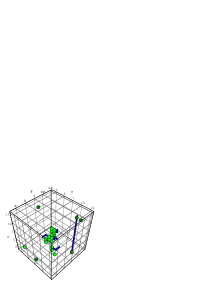
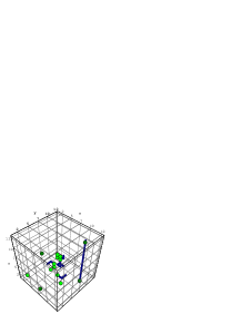
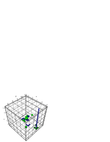
Figure 3:  Different definitions of the topological charge for a specific gluon configuration from Wilson action after $20$ cooling sweeps. The instantons reside at the same places for all definitions and are surrounded by monopoles. In this configuration a monopole loop wraps around the torus.

Fig. 4 presents a cooling history of a time slice of a gluon field. The topological charge using the Lüscher definition with the Wilson action is displayed for cooling steps 0, 15, 20 and 25. Without cooling the topological charge distribution cannot be identified with instantons due to quantum fluctuations. After 15-20 cooling steps one can assign instantons to clusters of topological charge. At cooling sweep 20 an instanton and an anti-instanton emerge. From cooling steps 35-40 they begin to approach each other and annihilate several steps later (not shown). Monopole loops also thin out with cooling, but they survive in the presence of instantons. In general, there is an enhanced probability that monopole loops are present in the vicinity of instantons in all gauge field configurations.

0 cooling sweeps	15 cooling sweeps
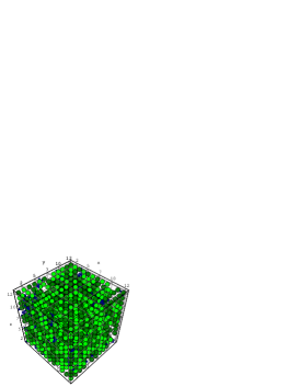
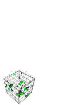
20 cooling sweeps	25 cooling sweeps

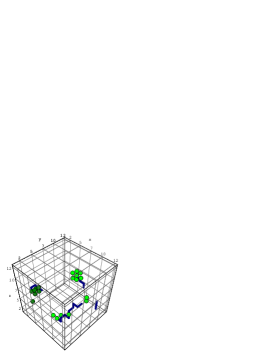
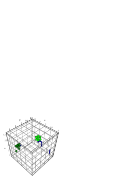
Figure 4:  Cooling history for a specific gauge field configuration from Wilson action at a fixed time slice. The dots represent the topological charge distribution in the Lüscher definition with $|q(x)|>0.01$. Positive (negative) charges are plotted with a light (dark) dot. The monopole loops correspond to lines. With cooling instantons evolve from noise accompanied by monopole loops in almost all cases. Note that time-like monopoles cannot be seen in these plots.

5 Conclusion

We computed average sizes of instantons and correlation functions between instantons and monopoles for different topological charge definitions, for different lattice actions, for cooled and constrained smoothed configurations. The auto-correlation functions between the topological charge density yield consistent results of instanton sizes for the Wilson and fix-point action. In the confinement phase the instanton size ranges from $\sigma=0.2-0.3$ fm whereas in the deconfinement phase $\sigma=0.1-0.2$ fm. The correlation functions between abelian monopoles and instantons are very similar for the geometrical and the field theoretical definition. They are hardly affected by cooling (Wilson action) or by constrained smoothing (fix-point action) and are qualitatively the same even across the deconfinement phase transition. The correlation length was found $\zeta=0.15-0.25$ fm in the confinement and $\zeta=0.25-0.35$ fm in the deconfinement phase.

We further calculated the local values of topological charges and monopole currents and directly displayed them with the help of computer graphics. After a few cooling sweeps one observes clearly that instantons are accompanied by monopole loops. This correlation occurs on all (semi-classical) gauge field configurations considered. In a cooling history we demonstrated how instantons evolve from fluctuating gauge fields and how they are surrounded by monopoles. Combining the above finding that the correlations are rather insensitive under cooling or smoothing together with that of the 3D images, we conclude that the topological charge goes hand in hand with monopoles also in the original gauge field configurations. The demonstration of our simulation together with analytical investigations [1, 14] might present a first indication of a deep relation between the topological structure of compact abelian and non-abelian gauge field theories. Since in abelian theories monopoles are responsible for confinement, and if such a relationship existed, this could be accepted as a topological proof of quark confinement.

6 Acknowledgments

We appreciate the cooperation with E.-M. Ilgenfritz and M. Müller-Preußker at Humboldt University Berlin where part of the work was done. We thank G. Schierholz who provided us with a routine to compute the Lüscher charge and W. Sakuler for continued interest. This work was partially supported by FWF under Contract No. P11456-PHY.

References

- [1] M.N. Chernodub and F.V. Gubarev, JETP Lett. 62 (1995) 100; R.C. Brower, K.N. Orginos and Chung-I Tan, hep-th/9610101.
- [2] A. Hart and M. Teper, Phys. Lett. B 371 (1996) 261; V. Bornyakov and G. Schierholz, Phys. Lett. B 384 (1996) 190; M. Fukushima, S. Sasaki, H. Suganuma, A. Tanaka, H. Toki and D. Diakonov, hep-lat/9608084.
- [3] S. Thurner, H. Markum and W. Sakuler, Proceedings of Confinement 95, Osaka 1995, eds. H. Toki et al. (World Scientific, 1996) 77 (hep-th/9506123); S. Thurner, M. Feurstein, H. Markum and W. Sakuler, Phys. Rev. D 54 (1996) 3457; M. Feurstein, H. Markum and S. Thurner, hep-lat/9608037.
- [4] T. DeGrand, A. Hasenfratz, P. Hasenfratz and F. Niedermayer, Nucl. Phys. B 454 (1995) 578; Nucl. Phys. B 454 (1995) 615.
- [5] M. Feurstein, E.-M. Ilgenfritz, M. Müller-Preußker and S. Thurner, hep-lat/9611024.
- [6] P. Di Vecchia, K. Fabricius, G.C. Rossi and G. Veneziano, Nucl. Phys. B 192 (1981) 392; Phys. Lett. B 108 (1982) 323; M. Campostrini, A. Di Giacomo and H. Panagopoulos, Phys. Lett. B 212 (1988) 206; M. Campostrini, A. Di Giacomo, H. Panagopoulos and E. Vicari, Nucl. Phys. B 329 (1990) 683.
- [7] A. Kronfeld, Nucl. Phys. B (Proc. Suppl.) 4 (1988) 329.
- [8] M. Lüscher, Commun. Math. Phys. 85 (1982) 39; I.A. Fox, J.P. Gilchrist, M.L. Laursen and G. Schierholz, Phys. Rev. Lett. 54 (1985) 749.
- [9] G. ’t Hooft, Nucl. Phys. B 190 (1981) 455.
- [10] A. Kronfeld, G. Schierholz and U.-J. Wiese, Nucl. Phys. B 293 (1987) 461.
- [11] T. DeGrand, A. Hasenfratz and Decai Zhu, Nucl. Phys. B 475 (1996) 321; Nucl. Phys. B 478 (1996) 349.
- [12] M. Göckeler, A.S. Kronfeld, M.L. Laursen, G. Schierholz and U.-J. Wiese, Phys. Lett. B 233 (1989) 192.
- [13] S. Hioki et al., Phys. Lett. B 272 (1991) 326; T. Suzuki et al., Nucl. Phys. B (Proc. Suppl.) 26 (1992) 441; J. Smit and A.J. van der Sijs, Nucl. Phys. B 355 (1991) 603.
- [14] N. Seiberg and E. Witten, Nucl. Phys. B 426 (1994) 19.