SWAT/97/149

MONTE CARLO STUDY OF THE 3D THIRRING MODEL

I review three different non-perturbative approaches to the three dimensional $N_{f}$-flavor Thirring model: the $1/N_{f}$ expansion, Schwinger-Dyson equations, and Monte Carlo simulation. Simulation results are presented to support the existence of a non-perturbative fixed point at a chiral symmetry breaking phase transition for $N_{f}=2$ and 4, but not for $N_{f}=6$. Spectrum calculations for $N_{f}=2$ reveal conventional level ordering near the transition.

1 Introduction

In this talk I will present work done in collaboration with Luigi Del Debbio and John Mehegan $\!{}^{{\bf?}}$. The Thirring model is a field theory of relativistic fermions interacting via a contact term between conserved currents. Its Lagrangian is written

$${\cal L}=\bar{\psi}_{i}(\partial{\!\!\!/}\,+m)\psi_{i}+{g^{2}\over{2N_{f}}}(\bar{\psi}_{i}\gamma_{\mu}\psi_{i})^{2},$$ (1)

where $\psi_{i},\bar{\psi}_{i}$ are taken to be 4 component spinors with flavor index $i$ running from 1 to $N_{f}$. Why is this an interesting model to study in three spacetime dimensions? Firstly, it appears that the expansion in powers of $1/N_{f}$ is exactly renormalisable for $2<d<4$, which in turn suggests an equivalence between the strong coupling limit of the Thirring model and the infra-red behaviour of $\mbox{QED}_{3}$. This result is essentially a perturbative one, albeit using a different expansion parameter; however non-perturbative studies using e.g. the Schwinger-Dyson approach suggest the model may exhibit dynamical symmetry breaking and have a non-trivial ultra-violet fixed point, of the type discussed by Miransky in the context of quenched $\mbox{QED}_{4}$ $\!{}^{{\bf?}}$, for $N_{f}$ less than some critical $N_{fc}<\infty$. At the proposed fixed point there would be no small dimensionless parameter in play; this is therefore a natural candidate for investigation by Monte Carlo simulation of the lattice-regularised model. In the following I will review each of these approaches, before presenting our results. Finally, it is worth mentioning that non-trivial fixed-point behaviour of $\mbox{QED}_{3}$ has been proposed to account for non-Fermi liquid behaviour in high $T_{c}$ superconductors $\!{}^{{\bf?}}$.

2 Three non-perturbative approaches

2.1 $1/N_{f}$ expansion

The Lagrangian (1) may be rewritten using a vector auxiliary field $A_{\mu}$:

$${\cal L}=\bar{\psi}_{i}(\partial{\!\!\!/}\,+m)\psi_{i}+{{ig}\over\surd{N_{f}}}A_{\mu}\bar{\psi}_{i}\gamma_{\mu}\psi_{i}+{1\over 2}A_{\mu}A_{\mu}.$$ (2)

In weak coupling perturbation theory, the vector propagator $D_{\mu\nu}(k)$ is simply $\delta_{\mu\nu}$; however to leading order in $1/N_{f}$ the vacuum polarisation bubble also contributes, with the result that $D_{\mu\nu}$ acquires momentum dependence $\!{}^{{\bf?}}$ $\!{}^{{\bf?}}$:

$$D_{\mu\nu}(k)=\left(\delta_{\mu\nu}-{{k_{\mu}k_{\nu}}\over{k^{2}}}\right){1\over{1-\Pi(k^{2})}}+\mbox{longitudinal},$$ (3)

with

$$\Pi(k^{2})=-{g^{2}\over{2\pi}}\left(m+{1\over{2\surd{k^{2}}}}(k^{2}-4m^{2})\tan^{-1}\left({\surd{k^{2}}\over{2m}}\right)\right).$$ (4)

This form can be examined in two limits. In the UV régime

$$\lim_{k^{2}\to\infty}D_{\mu\nu}(k^{2})=\left(\delta_{\mu\nu}-{{k_{\mu}k_{\nu}}\over{k^{2}}}\right){8\over{g^{2}\surd{k^{2}}}}.$$ (5)

The $1/k$ asymptotic behaviour has the effect of softening the contact term and thus decreasing the superficial degree of divergence associated with higher order diagrams containing internal vector lines, such as fermion self-energy, two-loop vacuum polarisation, etc. These divergences can be absorbed by a finite number of counterterms, essentially due to a novel application of Weinberg’s theorem, rendering the $1/N_{f}$ expansion renormalisable $\!{}^{{\bf?}}$. At lowest non-trivial order, the corrections coincide with those calculated in the IR limit of $\mbox{QED}_{3}$ $\!{}^{{\bf?}}$, giving the first hint that the two models may be related.

In the low-momentum régime, (3,4) can be used to find a pole condition and hence calculate the mass $M_{V}$ of the vector bound state. The result depends on the dimensionless combination $(mg^{2})$ $\!{}^{{\bf?}}$:

$$M_{V}=\cases{2m\left(1-2\exp\left(-{{2\pi}\over{mg^{2}}}\right)\right)&$mg^{2}\to 0$;\cr m\sqrt{{6\over{mg^{2}}}}&$mg^{2}\to\infty$.\cr}$$ (6)

Thus we identify a smooth crossover from a weakly coupled theory in which the vector is a weakly bound $f\bar{f}$ state to a strongly coupled one in which it is almost massless. To leading order in $1/N_{f}$ the $(\bar{\psi}\gamma_{\mu}\psi)^{2}$ interaction is a marginal operator. In the strong coupling limit $g^{2}\to\infty$ a massless vector mediates interaction between conserved currents, suggesting that in this limit the theory is identical to $\mbox{QED}_{3}$.

2.2 Schwinger-Dyson equations

The Schwinger-Dyson approach $\!{}^{{\bf?}}$ is to solve for the full fermion propagator $S_{F}^{-1}(k)=A(k)ik{\!\!\!/}\,+\Sigma(k)$ self-consistently, by finding integral equations for the functions $A$ and $\Sigma$. The most systematic analysis of the Thirring model $\!{}^{{\bf?}}$ exploits a hidden local symmetry of (2) to fix a non-local gauge in which the wavefunction renormalisation $A(k)\equiv 1$. The usual truncations of setting the full vector propagator to its leading order $1/N_{f}$ form (3) and the full vertex $\Gamma_{\mu}(p,q)$ to the bare vertex $ig\gamma_{\mu}/\sqrt{N_{f}}$ (i.e. the ladder approximation) are also employed. The resulting SD equation for $\Sigma(k)$ can be solved analytically in the limit $g^{2}\to\infty$.

In the chiral limit $m\to 0$, a non-trivial solution for $\Sigma(k)$ is found for small values of $N_{f}$, signalled by a non-vanishing order parameter, the chiral condensate $\langle\bar{\psi}\psi\rangle$:

$$\langle\bar{\psi}\psi\rangle\propto\Lambda^{2}\exp(-3\pi/\sqrt{\textstyle{N_{f}\over N_{fc}}-1}),$$ (7)

with $\Lambda$ a UV cutoff. This solution exists for $N_{f}<N_{fc}=128/3\pi^{2}\simeq 4.3$, implying that in the strong coupling limit, a separation of IR and UV scales allowing a continuum limit can only be made as $N_{f}\to N_{fc}$. The essentially singular behaviour is reminiscent of quenched $\mbox{QED}_{4}$ $\!{}^{{\bf?}}$. For finite $g^{2}$ there is no analytic solution, but it has been argued that the critical curve $N_{fc}(g)$ is smooth $\!{}^{{\bf?}}$, implying that non-trivial UV fixed points as $g^{2}\to g_{c}^{2}(N_{f})$ may exist for integer $N_{f}<N_{fc}$. The Thirring interaction has thus become relevant. It should be noted, however, that a different truncation procedure yields $N_{fc}=\infty$ $\!{}^{{\bf?}}$. It is therefore desirable to try an alternative non-perturbative approach to see if fixed points can be identified, and to get an independent estimate of $N_{fc}$.

2.3 Lattice formulation

The lattice action we have used is

$$S = \frac{1}{2}\sum_{x\mu i}\bar{\chi}_{i}(x)\eta_{\mu}(x)\left[\chi_{i}(x+\hat{\mu})-\chi_{i}(x-\hat{\mu})\right]+$$ (8)

$$m\sum_{xi}\bar{\chi}_{i}(x)\chi_{i}(x)+\frac{g^{2}}{2N}\sum_{x\mu ij}\bar{\chi}_{i}(x)\chi_{i}(x+\hat{\mu})\bar{\chi}_{j}(x+\hat{\mu})\chi_{j}(x)$$

where $i$ runs over $N$ flavors of one-component staggered fermion fields $\chi,\bar{\chi}$, and $\eta_{\mu}(x)$ are the space-dependent Kawamoto-Smit phases which are lattice analogues of the $\gamma$-matrices. We have simulated the models with $N=1,2$ and 3, proceeding by introducing a vector auxiliary on lattice links by analogy with (2). Alternative formulations are possible $\!{}^{{\bf?}}$; we have chosen (8) so that there is no gauge symmetry, and the highest interaction is four-point.

There are two aspects of the formulation (8) which require further discussion. Firstly, and slightly unexpectedly, the lattice interaction current is not exactly conserved, because it couples to $iA_{\mu}$ and not $\exp(iA_{\mu})$. This means that the lattice vacuum polarisation tensor is not transverse, which at leading order in $1/N_{f}$ results in an additive renormalisation of the inverse coupling $(1/g^{2})$ $\!{}^{{\bf?}}$:

$$g^{2}\mapsto g^{2}_{R}={g^{2}\over{1-{2\over 3}g^{2}}}.$$ (9)

We should thus expect to find the strong coupling limit at $g_{R}^{2}\to\infty$, i.e. $1/g^{2}\to 2/3$ (for $1/g^{2}<2/3$ the model is not unitary). It is clear that for small $N_{f}$, identifying the limit $g_{R}^{2}\to\infty$ numerically will be difficult in practice.

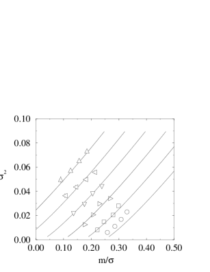
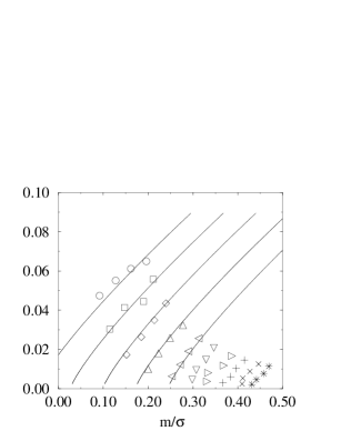
Figure 1:                                    Figure 2:

Secondly, when the lattice action (8) is recast in terms of physical fields $q,\bar{q}$ which have explicit spin and flavor indices, then we find $\!{}^{{\bf?}}$

(i) Each flavor of $\chi$ corresponds to 2 physical flavors, via fermion doubling, i.e.

$$N_{f}=2N.$$ (10)

(ii) In addition to the expected interaction term $(\bar{q}_{i}(\gamma_{\mu}\otimes 1\kern-4.5pt1)q_{i})^{2}$, where the second $2\times 2$ matrix in the product acts on flavor indices, (8) contains other interactions such as $(\bar{q}_{i}(\gamma_{5}\gamma_{\mu}\otimes 1\kern-4.5pt1)q_{i})^{2}$ and even non-covariant ones such as $(\bar{q}_{i}(\gamma_{4}\gamma_{\nu}\gamma_{\mu}\otimes\tau_{\nu}^{*})q_{i})^{2}$. These undesired terms are not suppressed in the limit lattice spacing $a\to 0$. Since a strongly-coupled theory requires a non-perturbative regularisation, we must take a robust attitude to this problem, and determine the fixed point behaviour, if any, by numerical measurement of critical scaling and spectral quantities.

3 Numerical results

3.1 Critical scaling

We have Monte Carlo data from lattice sizes $8^{3}$, $12^{3}$ and $16^{3}$, and a range of bare masses $ma=0.05,\ldots,0.01$ $\!{}^{{\bf?}}$. To determine the critical properties requires an extrapolation to the chiral limit $m\to 0$; this is best done globally, so in the neighbourhood of the chiral phase transition we assume an equation of state of the form

$$m=A\left({1\over g^{2}}-{1\over g_{c}^{2}}\right)\langle\bar{\psi}\psi\rangle^{\delta-1/\beta}+B\langle\bar{\psi}\psi\rangle^{\delta}.$$ (11)

Here $\delta$ and $\beta$ are standard critical exponents, which in a mean field treatment would assume the values $\delta=3$, $\beta={1\over 2}$. It follows that in the mean-field case a plot of $\langle\bar{\psi}\psi\rangle^{2}$ vs. $m/\langle\bar{\psi}\psi\rangle$, known as a Fisher plot, would yield straight lines for constant $1/g^{2}$ which would pass through the origin at the critical coupling, and above or below the origin in the super- or sub-critical region respectively. In Figs. 1 and 2 we show Fisher plots for $N_{f}=2$ in the neighbourhood of $1/g_{c}^{2}\simeq 1.9$ and $N_{f}=4$ near $1/g_{c}^{2}\simeq 0.6$. The lines denote our best fits to (11) assuming $\delta-1/\beta=1$, which follows from the ladder approximation $\!{}^{{\bf?}}$. The curvature indicates a slight departure from mean-field scaling. Our fits, which include a finite volume scaling analysis for $N_{f}=2$, are presented in Tab. 1

Table 1: Fits to the Equation of State

	$N_{f}=2$	$N_{f}=4$
$1/g_{c}^{2}$	1.92(2)	0.66(1)
$\delta$	2.75(9)	3.43(9)

The remaining exponents can be derived using the constraint between $\delta$ and $\beta$, and hyperscaling. The most significant result is not so much that the value of $\delta$ departs from the mean-field value in each case, but rather that the values from each model are distinct. This is consistent with the $N_{f}=2,4$ theories belonging to different universality classes.

A Fisher plot for $N_{f}=6$, shown in Fig. 3, shows no evidence for a chirally broken phase, and no fit of the form (11) is possible. Thus the data, from admittedly small lattices to date, strongly suggest

$$N_{fc}<6.$$ (12)

3.2 Spectroscopy

We have measured the physical fermion and bound state masses for $N_{f}=2$ on a $16^{3}$ lattice with $ma=0.01$. Fig. 4 shows fermion, pion and scalar masses vs. $1/g^{2}$, showing a sharp crossover near $1/g^{2}_{c}\simeq 1.9$. In the symmetric phase both pion and scalar look like weakly bound $f\bar{f}$ states, while in the broken phase the pion is the lightest particle, consistent with Goldstone’s theorem. There is no evidence for the absence of light bound states in the symmetric phase, predicted if the fixed point is described by an essential singularity $\!{}^{{\bf?}}$. We have also examined the vector channel, where the simplest interpolating operator projects onto states with both vector ($\bar{q}\gamma_{\mu}q$) and axial vector ($\bar{q}\gamma_{5}\gamma_{\mu}q$) quantum numbers. Surprisingly, we found both states to be light in the symmetric phase, even though to leading order in $1/N_{f}$ there is no bound state in the axial vector channel. This is a hint that the $1/N_{f}$ expansion may be failing to describe the physics even of the symmetric phase near the fixed point. Measurements in the broken phase are much noisier, but there is tentative evidence that the vector mass increases sharply.

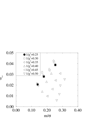
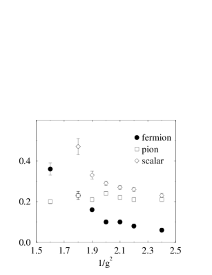
Figure 3:                                    Figure 4:

4 Summary

Our main results are that for $N_{f}=2,4$ there is clear evidence for a continuous chiral phase transition, with scaling described by distinct critical exponents in each case. No such transition is seen for $N_{f}=6$, implying $N_{fc}<6$. For $N_{f}=2$, we see conventional level ordering of the spectrum in fermion, pion and scalar channels across the transition, and light states in the symmetric phase in both vector and axial vector channels.

References

References

- [1] L. Del Debbio and S.J. Hands, Phys. Lett. B 373, 171 (1996); L. Del Debbio, S.J. Hands and J.C. Mehegan, hep-lat/9701016 (1997).
- [2] P.I. Fomin, V.P. Gusynin, V.A. Miransky and Yu. A. Sitenko, Riv. Nuovo Cimento 6, 1 (1983); V.A. Miransky, Nuovo Cimento A 90, 149 (1985).
- [3] I.J.R. Aitchison and N.E. Mavromatos, Phys. Rev. B 53, 9321 (1996); N.E. Mavromatos, these proceedings.
- [4] G. Parisi, Nucl. Phys. B 100, 368 (1975); S. Hikami and T. Muta, Prog. Theor. Phys. 57, 785 (1977).
- [5] M. Gomes, R.S. Mendes, R.F. Ribeiro and A.J. da Silva, Phys. Rev. D 43, 3516 (1991).
- [6] S.J. Hands, Phys. Rev. D 51, 5816 (1995).
- [7] D. Espriu et al, Z. Phys. C 13, 153 (1982); A. Palanques-Mestre and P. Pascual, Comm. Math. Phys. 95, 277 (1984).
- [8] T. Itoh, Y. Kim, M. Sugiura and K. Yamawaki, Prog. Theor. Phys. 93, 417 (1995).
- [9] K.-I. Kondo, Nucl. Phys. B 450, 251 (1995).
- [10] D.K. Hong and S.H. Park, Phys. Rev. D 49, 5507 (1994).
- [11] S. Kim and Y. Kim, hep-lat/9605021 (1996); Y. Kim, these proceedings.
- [12] E. Dagotto et al, Nucl. Phys. B 347, 217 (1990).
- [13] V.A. Miransky and K. Yamawaki, hep-th/9611142 (1996); V.A. Miransky, these proceedings.