CELLULAR AUTOMATA AND SELF ORGANIZED CRITICALITY

Abstract

Cellular automata provide a fascinating class of dynamical systems capable of diverse complex behavior. These include simplified models for many phenomena seen in nature. Among other things, they provide insight into self-organized criticality, wherein dissipative systems naturally drive themselves to a critical state with important phenomena occurring over a wide range of length and time scales.

1 Self-organized Criticality

Self-organized criticality is a concept aimed at describing a class of dynamical systems which naturally drive themselves to a state where interesting physics occurs on all scales[1]. The idea provides a possible “explanation” of the omnipresent multi-scale structures throughout the natural world, ranging from the fractal structure of mountains, to the power law spectra of earthquake sizes [2]. Recent applications include such diverse topics as punctuated evolution [3] and traffic flow [4]. The concept has even been invoked to explain the unpredictable nature of economic systems, i.e. why you can’t beat the stock market [5].

The prototypical example is a sandpile. On slowly adding grains of sand to an empty table, a pile will grow until its slope becomes critical and avalanches start spilling over the sides. If the slope becomes too large, a large catastrophic avalanche is likely, and the slope will reduce. If the slope is too small, then the sand will accumulate to make the pile steeper. Ultimately one should obtain avalanches of all sizes, with the prediction of the size for the next avalanche being impossible without actually running the experiment.

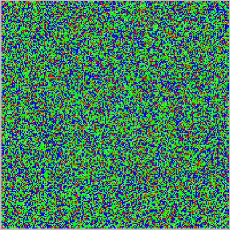
Figure 1: The sandpile model in the final stable state after adding lots of sand to random places. The lattice is 198 cells by 198 cells. The color code is grey, red, blue, and green for heights 0,1,2, and 3, respectively. Despite the lack of obvious patterns, subtle correlations are present; for example no two adjacent sites have height zero.

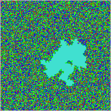
a.     b.

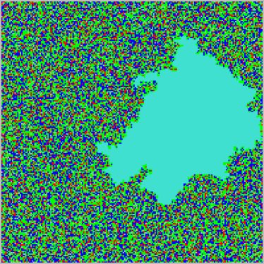
Figure 2: An avalanche obtained by adding a small amount of sand to the configuration in Fig. 1. Stable sites which have tumbled during the avalanche are distinguished by being colored light blue. The still active sites on the left image are colored yellowish brown. The image on the right is the final state after the avalanche has ended. Note that the final avalanche region is simply connected. This is a general result proven later in the text.

Self-organized criticality nicely compliments the concept of chaos. In the latter, dynamical systems with a few degrees of freedom, say three or more, can display highly complex behavior, including fractal structures. With self-organized criticality, we start instead with systems of many degrees of freedom, and find a few general common features. Another attractive feature of this topic is the ease with which computer models can be implemented and the elegance of the resulting graphics. Most of the figures in this chapter were produced using my publicly available set of programs “xtoys”[6].

The original Bak, Tang, Wiesenfeld paper [1] presented a simple model wherein each site in a two dimensional lattice has a state represented by a positive integer $z_{i}$. This integer can be thought of as representing the amount of sand at that location, or in another sense it represents the slope of the sandpile at that point. Neither of these analogies is fully accurate, for the model has aspects of each.

The dynamics follows by setting a threshold $z_{T}$ above which any given $z_{i}$ is unstable. Without loss of generality, I take this threshold to be $z_{T}=3$. Time now proceeds in discrete steps. In one such step each unstable site “tumbles” or “topples,” dropping by four and adding one grain to each of its four nearest neighbors. This may produce other unstable sites, and thus an avalanche can ensue for further time steps until all sites are stable. Fig. 1 shows a typical configuration on a 198 by 198 lattice after lots of random sand addition followed by relaxation. Fig. 2 shows an avalanche proceeding on this lattice.

A natural experiment consists of adding a grain of sand to a random site and measuring the number of topplings and the number of time steps for the resulting avalanche. Repeating this many times to gain statistics, the distribution of avalanche sizes and lengths displays a power law behavior, with all sizes appearing. In Ref. [7] such experiments showed that the distribution of the number of tumbling events $s$ in an avalanche empirically scales as

$$P(s)\sim s^{-1.07}$$

and the number of time steps $\tau$ for avalanches scales as

$$P(\tau)\sim\tau^{-1.14}$$

This model has been extensively studied analytically. While as yet there is no exact calculation of these exponents, a lot is known. In particular, the critical ensemble is well characterized. I will return to these points later.

The extent to which laboratory experiments reproduce these phenomena is somewhat controversial. A recent study of avalanche dynamics [8] in rice piles showed power laws with long-grain rice, but more ambiguous results followed similar experiments with short-grain rice.

2 Cellular Automata

The sandpile model is a simple example of a cellular automaton system[9, 10]. Each site or “cell” of our lattice follows a prescribed rule evolving in discrete time steps. At each step, the new value for a cell depends only on the current state of itself and its neighbors. These systems are fascinating in that deceptively simple rules can give rise to extremely complex behavior. Furthermore, slight changes in the rules can dramatically change their behavior.

Even though the formulation of a cellular automaton may seem almost trivial, there are a huge number of possible rules. For example, suppose I consider two dimensional models where each cell can take only one of two possible states. These might be referred to as unset or set bits, or more figuratively as “dead” or “alive.” Suppose furthermore that I restrict myself to rules where the evolution of a given cell to the next time step depends only on the current values of the cell and each of its eight nearest neighbors. In this case there are $2^{9}=512$ possible arrangements around a cell, and a general rule needs to specify the next state for each of these arrangements. This gives $2^{512}=1.3\times 10^{154}$ possible rules. Given that the universe is only of order $3\times 10^{17}$ seconds old, clearly only a vanishing fraction of these rules have a chance of being studied in any of our lifetimes.

A simple subset of rules called “totalistic” have the state of the updated cell only depend on the total number of living neighbors. With the eight cell neighborhood, there are nine possible values for this sum, and the new value for the cell requires specification of the new state for each of these as well as for the current state of the cell. This gives $2^{18}=262,144$ rules; still large, but not truly astronomical. If I restrict the rule to depending on the total of only the four nearest neighbors, I then have a modest $2^{10}=1024$ cases to consider. Other than the sandpile model, most of the following will be restricted to such totalistic rules.

With a discrete set of states, cellular automata have the appealing feature of being easily implementable entirely by logical operations, the natural functions of computer circuitry. Also, the state of several cells can be stored and manipulated within a single computer word. Using such tricks, these models can often be implemented to run extremely fast, leading to hope that such models may supply simulation methods as good as or better than the conventional use of floating point fields on a discrete grid. With this motivation, considerable attention has been paid to cellular automata that may simulate fluid flow. Another advantage of this approach is the ability to work with arbitrary boundary conditions. These topics go beyond the scope of this article. A nice review can be found in Ref. [11]

3 Conway’s Life

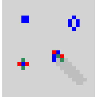
Figure 3: Some living configurations in life. The top two are stable patterns. The lower left shows a “blinker” or “traffic light” which oscillates with a period of two. On the lower right is a glider, which propagates diagonally through the lattice. Blue denotes a state that is and just was alive, red is newborn, and green represents just died. The track of the glider is darkened slightly over the remaining grey background.

       

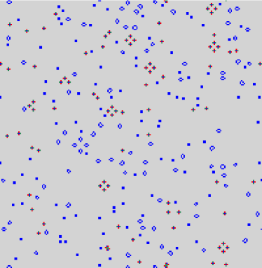
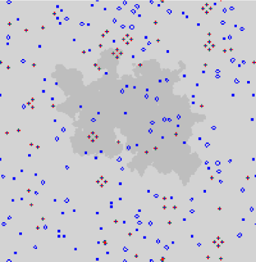
Figure 4: On the left is a configuration in life resulting from a random start and evolved until only stable and period two oscillators remain. On the right is the state after a small disturbance was introduced in the center and allowed to die out. Note the irregular shape of the disturbed region, which has been tinted a darker grey. The lattice here is 198 sites wide by 202 sites high, with periodic boundaries.

Perhaps the most famous cellular automaton system is Conway’s “Game of Life” [12]. For this there exists a vast literature; so, I will only mention a couple of interesting features. The rule involves the eight cell neighborhood, and if a cell is initially “dead” it becomes alive if and only if it has exactly three live neighbors, or “parents.” A living cell dies of loneliness if it has less than two live neighbors, and of overcrowding if it has more than three live neighbors. Only in the case of exactly two or three live neighbors does it survive.

While simple to state, this model displays fascinating complexity. There are simple isolated sets of live cells that quietly survive, such as a block of four neighboring live cells forming a two by two square. Other configurations oscillate, such as three live cells in a row, which alternate between being vertically and horizontally oriented. A particularly amusing local configuration has five live cells; say starting with coordinates $\{(0,0),(0,1),(0,2),(1,2),(2,1)\}$. After four time steps this configuration returns to its original shape, but displaced by $(-1,1)$. On an otherwise empty board, this “glider” continues to propagate as a single entity. In an on-screen simulation, it appears much as a small insect crawling about. Some elementary configurations are shown in Fig. 3. A large collection of fascinating complex life configurations can be found at [13].

Figure 5: The distribution of avalanches generated by adding gliders randomly to a system in the game of life consisting of stable and period two oscillators. An avalanche occupies the period until the system has relaxed again into such a periodic state. The solid line represents 25,000 avalanches on a 512 by 512 lattice, and the dashed line is for 6,000 avalanches on a 1024 by 1024 system. This figure is taken from Ref. [15].

Gliders allow information to be propagated over long distances, and it has been proven that with a complicated enough initial configuration, one can construct a computer out of live cells on a life board [12]. Special sub-configurations form the analog of electronic gates, which can control beams of gliders representing bits. Indeed, since life is capable of universal computation, one might imagine a life board programmed to simulate, say the game of life.

There is some limited evidence that the game of life also displays self-organized criticality [14, 15]. One can repeatedly throw down gliders, which collide and create a background of static and oscillating clumps. While oscillators of arbitrarily long period are known to exist, those with period longer than two are extremely rare and almost never created from unorganized initialization. Once the system has settled into a loop, then another glider can be tossed on, giving a disturbance. An avalanche is defined to occur during the period until the system again goes into an oscillating state. Fig. 4 shows the effect of such a disturbance. In Fig. 5 I show the distribution of such avalanches as measured on modest lattices. There is a hint of a power law superposed on additional structure from avalanches of only a few time steps, and a rounding at large times possibly due to finite size effects. The criticality of life remains controversial; Ref. [16] has looked unsuccessfully for a power law distribution of activity as one moves in from a source on the boundary. The relation between these two experiments is unclear.

4 Fredkin’s modulo two rule

A simple but highly amusing rule takes at each time step the “exclusive or” (XOR) operation between a site and its neighbors. This rule has the remarkable property of self replication [17]. Starting with any given initial pattern, after $2^{n}$ time steps copies of the original state occupy positions separated by $2^{n}$ spatial sites from the original in every direction as specified in the chosen neighborhood. In Fig. 6 I show an example of this with the four cell neighborhood.

In this rule, the pattern is generally rather complex just before returning to the replicated case, i.e. after $2^{n}-1$ steps. Fig. 7 shows the pattern obtained from a single set pixel after this rule has been applied for 63 time steps using the four nearest cells as the neighborhood. Note the fractal structure. In one more time step, all but five copies of the original set bit die.

       

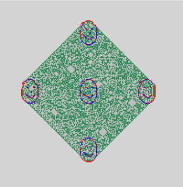
Figure 6: Starting from the initial configuration on the left, the modulo two rule is evolved using the four nearest neighbors. At a certain stage, five copies of the original image appear. The green denotes just expired cells, which form a complex fractal pattern which has just decayed into the five copies.

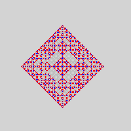
Figure 7: The state after applying 63 steps of the modulo two rule using the four nearest neighbors to an initial state of a single set bit. After the next time step this fractal structure decays into only five remaining live cells.

Unlike most cellular automaton rules, this gives a dynamics which in some sense is not really “complex.” In most cases the simplest way to predict the evolution of a cellular automaton rule is to actually run it. Here, however, I have an easier way to predict what the final pattern will look like; it is always an XOR operation between several displaced copies of the configuration that appeared $2^{n}$ time steps in the past. Despite the lack of complexity, this rule shows rather dramatically that cellular automata are indeed capable of “reproduction.”

5 Reversible rules

Reversibility is rather elusive among cellular automata. In the game of life, a single isolated cell immediately dies leaving no trace; thus it is impossible from the state at a given time to reconstruct what was there one time step back. A related difficult problem is to construct “garden of Eden” configurations which are impossible to arrive at from any previous state.

Fredkin pointed out an interesting class of reversible rules based on an analogy with molecular dynamics [10]. In the later one specifies both the position and the velocities of a set of particles and evolves the system under Newton’s equations with some given inter-particle force law. Reversal can then be accomplished by merely changing the signs of all the velocities.

In a cellular automaton an analog of velocity requires the value of the cells at two successive time steps. Based on this, Fredkin presented a very simple scheme using the previous state to generate a wide class of reversible rules. He considered taking an arbitrary automaton rule at a given time, and then added an exclusive or (XOR) operation of the result with the state one step back in time. These combined operations could then be reversed by merely interchanging two successive time steps, the analogy of reversing the velocities.

To see this more mathematically, suppose the state at time $i$ is $s_{i}$, and the underlying rule begins by taking some arbitrary function $f(s_{i})$. Then the full rule takes for the next time step $s_{i+1}=f(s_{i})\ {\rm XOR}\ s_{i-1}$. Here the exclusive or operation is taken site by site over the entire lattice. Elementary properties of the XOR operation then give $s_{i-1}=f(s_{i})\ {\rm XOR}\ s_{i+1}$, which is the identical rule for the time reversed dynamics.

These rules provide a wonderful way to play with the concepts of entropy and reversibility. Indeed, an idealized universe of cellular automata enables experiements which would be impossible to carry out in the real world. In Fig. 8 I show the evolution of a simple image under such a rule. The experiment is a crude simulation of a coffee cup shattering after being dropped on the floor. After a few steps it appears quite randomized. Reversal of the momenta of all relevant atoms in the coffee cup would allow its reconstruction. In the model this is easily accomplished by swapping two time steps. After reversal, continuing with the same rule reconstructs the original image. At all stages the “information” contained in the system must be constant, even though the image may appear of drastically different complexity.

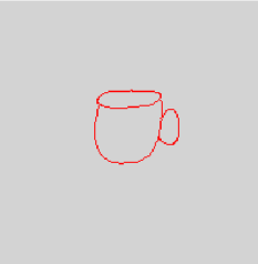
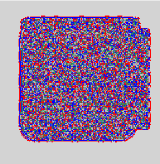
a.     b.     c.

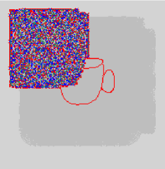
Figure 8: The encryption of a coffee cup. The original rule uses the eight cell neighborhood with births on 1,3,4, and 7 neighbors and survivors on 0,2,3,4, and 8 neighbors. The rule is modified by XOR’ing the result with the cell one time step back. Swapping two adjacent time steps will bring the encrypted coffee cup back exactly. The third image is what happens if you reverse the process except make an error on one bit in the upper left hand quadrant. Note the effect of a “speed of light” in the problem.

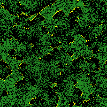
a.    b.

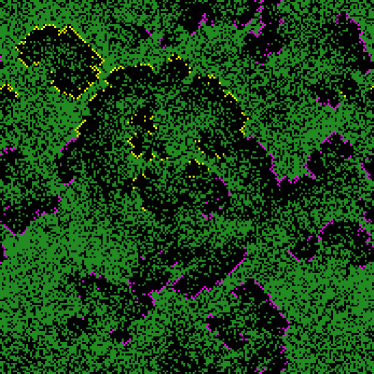
Figure 9: On the left is a snapshot of the forest fire model on a 198 by 198 lattice. Trees are continuously burning at a slow rate, while fires burn them down and spread to nearest neighbor trees. Here the four cell neighborhood is used. On the right is a variation where two species of bunnies are competing to eat a common grass. The yellow and purple colors here distinguish the parity of the site plus time step. Eventually one of the two species dominates and the other dies out.

The reconstruction process is highly sensitive to the reversal being precise. The analog here is to the sensitivity to initial conditions in dynamical systems. In Fig. 8c I try to reproduce the coffee cup from its shards as in the above experiment, except that now at the time of reversal I modify the state of exactly one pixel. The reversal process recovers the original image only in regions outside the “light cone” for the modified pixel. As the disturbance can only propagate to neighbors in one time step, pixels outside $n$ steps can not know of the change before an equal number of time steps. This use of an XOR operation to generate reversible complex mappings is an integral part of the Data Encryption Standard; see, for example, Ref. [18].

6 Forest fires and bunny wars

An amusing model of forest fires has three possible states per cell, empty, a tree, or a fire. For the updating step, any empty site can have a tree born with a small probability. At the same time, any existing fire spreads to neighboring trees leaving its own cell empty. The rule here differs from those discussed previously in having a stochastic nature. As the system is made larger, the growth rate for the trees should decrease to just enough to keep the fires going.

If too many trees grow, one obtains a large fire reducing their density, while if there are too few trees, fires die out. On a finite system, one should light a fire somewhere to get the system started. On the other hand, as the system becomes larger, the growth rate for the trees can be reduced without the fire expiring. In a steady state the system has fire fronts continually passing through the system, as illustrated in Fig. 9a.. Perhaps there is a moral here that one should be careful about extinguishing all fires in the real world, for this may enhance the possibility for a catastrophic uncontrollable fire. It is not entirely clear whether this model is actually critical. What seems to happen on large systems is that stable spiral structures form and set up a steady rotation. For a review of this and several related models, see Ref. [19].

A variation on this model has several “species” of fires. Perhaps a better metaphor is to think of different species of bunny, competing for the same slowly growing food resource. With the four cell neighborhood, a natural division into species is given by the parity of the site plus the time step. Fig. 9b. shows a state in the evolution of such a model when both species are present. This situation, however, is highly unstable, with any fluctuation favoring one species tending to grow until the competitor is eliminated. This model provides a discrete realization of the “principle of competitive exclusion” in biological systems [20]. Stability of a species requires that it occupy its own niche and not compete for exactly the same resources as another.

7 The sandpile revisited

Very little is known analytically about general cellular automata. However, in a series of papers, Deepak Dhar and co-workers have shown that the sandpile model has some rather remarkable mathematical properties [21, 22, 23, 24]. In particular, the critical ensemble of the system has been well characterized in terms of an Abelian group. In the following I will generally follow the discussion given in Refs. [25, 2].

Dhar introduced the useful toppling matrix $\Delta_{i,j}$ with integer elements representing the change in the height, $z$ at site $i$ resulting from a toppling at site $j$ [21]. More precisely, under a toppling at site $j,$ the height at any site $i$ becomes $z_{i}-\Delta_{i,j}$. For the simple two dimensional sand model the toppling matrix is thus

$$\matrix{\Delta_{i,j}&=4&i=j\cr\Delta_{i,j}&=-1&i,j{\rm\ \ nearest\ neighbors}\cr\Delta_{i,j}&=0&{\rm\ \ otherwise.}\cr}$$

For this discussion there is little special to the specific lattice geometry; indeed, the following results easily generalize to other lattices and dimensions. The analysis requires only that under a toppling of a single site $i,$ that site has its slope decreased $(\Delta_{i,i}>0)$, the slope at any other site is either increased or unchanged $(\Delta_{i,j}\leq 0,j\neq i)$, the total amount of sand in the system does not increase $(\sum_{j}\Delta_{i,j}\geq 0)$, and, finally, that each site be connected through toppling events to some location where sand can be lost, such as at a boundary.

For the specific case in Eq. 3, the sum of slopes over all sites is conserved whenever a site away from the lattice edge undergoes a toppling. Only at the lattice boundaries can sand be lost. Thus the details of this model depend crucially on the boundaries, which we take to be open. A toppling at an edge loses one grain of sand and at a corner loses two.

The actual value of the maximum stable height $z_{T}$ is unimportant to the dynamics. This can be changed by simply adding constants to all the $z_{i}$. Thus without loss of generality I consider $z_{T}=3$. With this convention, if all $z_{i}$ are initially non-negative they will remain so, and I thus restrict myself to states $C$ belonging to that set. The states where all $z_{i}$ are positive and less than 4 are called stable; a state that has any $z_{i}$ larger than or equal to 4 is called unstable. One conceptually useful configuration is the minimally stable state $C^{*}$ which has all the heights at the critical value $z_{T}$. By construction, any addition of sand to $C^{*}$ will give an unstable state leading to a large avalanche.

I now formally define various operators acting on the states $C$. First, the “sand addition” operator $\alpha_{i}$ acting on any $C$ yields the state $\alpha_{i}C$ where $z_{i}=z_{i}+1$ and all other $z$ are unchanged. Next, the toppling operator $t_{i}$ transforms $C$ into the state with heights $z^{\prime}_{j}$ where $z^{\prime}_{j}=z_{j}-\Delta_{i,j}$. The operator $U$ which updates the lattice one time step is now simply the product of $t_{i}$ over all sites where the slope is unstable,

$$UC=\prod_{i}t_{i}^{p_{i}}C$$

where $p_{i}=1$ if $z_{i}\geq 4$; $0$ otherwise. Using $U$ repeatedly gives the relaxation operator $R$. Applied to any state $C$ this corresponds to repeating $U$ until no more $z_{i}$ change. Neither $U$ nor $R$ have any effect on stable states. Finally, I define the avalanche operators $a_{i}$ describing the action of adding a grain of sand followed by relaxation

$$a_{i}C=R\alpha_{i}C.$$

At this point it is not entirely clear that the operator $R$ exists; in particular, it might be that the updating procedure enters a non-trivial cycle consisting of a never ending avalanche. I now prove that this is impossible. First note that a toppling in the interior of the lattice does not change the total amount of sand. A toppling on the boundary, however, decreases this sum due to sand falling off the edge. Thus, during an avalanche the total sand in the system is a non-increasing quantity. No closed cycle can have toppling at the boundary since this will decrease the sum. Next, the sand on the boundary will monotonically increase if there is any toppling one site further in. This also can not happen in a cycle; thus, there can be no topplings one site away from the edges. By induction there can be no toppling arbitrary distances in from the boundary; thus, there can be no cycle, and the relaxation operator exists. Note that for a general geometry this argument requires that every site be eventually connected to an edge where sand can be lost.

With an edge less system, such as under periodic boundaries, no sand would be lost and thus cycles are expected and easily observed. These models might be called “Escher models” after the artist constructing drawings of water flowing perpetually downhill and yet circulating in the system. While little is known about the dynamics of this variation on the sandpile model, some studies have been done under the nomenclature of “chip-firing games” [26]. A recent paper [27] has argued that this lossless sandpile model on an appropriate lattice is capable of universal computation.

I now introduce the concept of recursive states. This set, denoted ${\cal R}$, includes those stable states which can be reached from any stable state by some addition of sand followed by relaxation. This set is not empty because it contains at least the minimally stable state $C^{*}$. Indeed, that state can be obtained from any other by carefully adding just enough sand to each site to make $z_{i}$ equal to three. Thus, one might alternatively define ${\cal R}$ as the set of states which can be obtained from $C^{*}$ by acting with some product of the operators $a_{i}$.

It is easily shown that there exist non-recursive, transient states; for instance, no recursive state can have two adjacent heights both being zero. If you try to tumble one site to zero height, then it drops a grain of sand on its neighbors. If you then tumble a neighbor to zero, it dumps a grain back on the original site. One can also show that the self-organized critical ensemble, reached under random addition of sand to the system, has equal probability for each state in the recursive set. This is a consequence of the Abelian nature of this system, as discussed below.

The crucial results of Refs. [21, 22, 23, 24] are that the operators $a_{i}$ acting on stable states commute, and they generate an Abelian group when restricted to recursive states. I begin by showing that the operators commute, that is $a_{i}a_{j}C=a_{j}a_{i}C$ for all $C$. First I express the $a$’s in terms of toppling and adding operators

$$a_{i}a_{j}C=\left(\prod_{k=1}^{n_{1}}t_{l_{k}}\right)\alpha_{i}\left(\prod_{k=n_{1}+1}^{n}t_{l_{k}}\right)\alpha_{j}C$$

where the specific number of topplings $n_{1}$ and $n$ depend on $i,$ $j,$ and $C$. Acting on general states, the operators $t$ and $\alpha$ all commute because they merely linearly add or subtract heights. Therefore I can shift $\alpha_{i}$ to the right in this expression:

$$a_{i}a_{j}C=\left(\prod_{k=1}^{n}t_{l_{k}}\right)\alpha_{i}\alpha_{j}C$$

Now I rearrange the product of topplings. In the non-trivial case that the $\alpha$-operators render either $i$ or $j$ (or both) unstable, the product must contain toppling operators corresponding to those unstable sites. I shift those operators to the right. Those operators constitute by definition the update operator, U, so I can write

$$a_{i}a_{j}C=\left(\prod t_{l_{k}}\right)U\alpha_{i}\alpha_{j}C$$

The factors within the bracket are the remaining $t$’s. Now, the update operator may leave some sites still unstable, and then the product must include further toppling operators; working on those sites, I can pull out another factor of the update operator. This procedure can be repeated until I have used all the toppling factors and the state is stable. Thus, I can identify the operator within the brackets in Eq. (8) as the relaxation operator $R$. But $\alpha_{i}\alpha_{j}C$ is the same state as $\alpha_{j}\alpha_{i}C$, so $a_{i}a_{j}C=a_{j}a_{i}C$.

A trivial consequence of this argument is that the total number of tumbling events occurring in the operations $a_{i}a_{j}C$ and $a_{j}a_{i}C$ are the same. Of course, if a particular site $k$ tumbles it can be caused by either addition; the orders of the tumbling events may or may not be altered.

An intuitive argument that sand addition may be commutative uses an analogy with combining many digit numbers under long addition. The tumbling operation is much like carrying, except rather than to the next digit the overflow spreads to several neighbors. As addition is known to be Abelian, despite the confusing elementary-school rules, I might expect the sandpile addition rule also to be.

I now prove that the avalanche operators have unique inverses when restricted to recursive states; that is, there exists a unique operator $a_{i}^{-1}$ such that $a_{i}(a_{i}^{-1}C)=C$ for all $C$ in $\cal R$. This implies that the operators $a_{i}$ acting on the recursive set generate an Abelian group. For any recursive state $C$ I first find another recursive state such that $a_{i}$ acting on it gives $C$, and I then show that this construction is unique.

I begin by adding a grain of sand at site $i$ to the state $C$ and then relax the system. This generates a new recursive state $a_{i}C$. Now since the state $C$ is by assumption recursive, there is some way to add sand to regenerate $C$ from any given state. In particular, there is some product $P$ of addition operators $a_{j}$ such that

$$C=Pa_{i}C$$

But the $a$’s commute, so I have

$$C=a_{i}PC$$

and thus $PC$ is a recursive state on which $a_{i}$ gives $C$.

I must now show that this state is unique. Consider repeating the above process to find a series of states $C_{n}$ satisfying

$$(a_{i})^{n}C_{n}=C.$$

Because on a finite system the total number of stable states is finite, the sequence of states $C_{n}$ must eventually enter a loop. I can run backwards around this loop by adding back the sand repeatedly to the given site. As the original state $C$ appears in resupplying the sand, $C$ itself must itself belong to the loop. Calling the length of the loop $m$, I have $(a_{i})^{m}C=C$. I now uniquely define $a_{i}^{-1}C=a_{i}^{m-1}C$.

I now have sufficient machinery to count the number of recursive states. As all such can be obtained by adding sand to $C^{*}$ , I can write any state $C\in{\cal R}$ in the form

$$C=\left(\prod_{i}a_{i}^{n_{i}}\right)C^{*}.$$

Here the integers $n_{i}$ represent the amount of sand to be added at the respective sites. However, in general there are several different ways to reach any given state. In particular, adding four grains of sand to any one site must force a toppling and is equivalent to adding a single grain to each of its neighbors. This can be expressed as the operator statement

$$a_{i}^{4}=\prod_{j\in nn}a_{j}$$

where the product is over the nearest neighbors to site $i$. I can rewrite this equation by multiplying by the product of inverse avalanche operators on the nearest neighbors on both sides, thus obtaining for any site $i$

$$\prod_{j}a_{j}^{\Delta_{ij}}=E$$

where $E$ is the identity operator. This allows me to shift the powers appearing in Eq. (12). Define $N$ to be the number of sites in the system. If I label states by the vector ${\bf n}=(n_{1},n_{2},n_{3},\ldots n_{N})$ I see that two states are equivalent if the difference of these vectors is of the form $\sum_{j}\beta_{j}\Delta_{ij}$ where the coefficients $\beta_{j}$ are integers. These are the only constraints; if two states can not be related by toppling they are independent. Thus any vector ${\bf n}$ can be translated repeatedly until it lies in an $N$-dimensional hyper-parallelepiped whose base edges are the vectors $\Delta_{ji}$, $j=1,\ldots N.$ The vertices of this object have integer coordinates and its volume is the number of integer coordinate points inside it. This volume is just the absolute value of the determinant of $\Delta$ . Thus the number of recursive states equals the absolute value of the determinant of the toppling matrix $\Delta$.

For large lattices this determinant can be found easily by Fourier transform. In particular, whereas there are $4N$ stable states, there are only

$$\exp\left(N\int_{(-\pi,-\pi)}^{(\pi,\pi)}{d^{2}q\over(2\pi)^{2}}\ln(4-2q_{x}-2q_{y})\right)\simeq(3.2102..)^{N}$$

recursive states. Thus starting from an arbitrary state and adding sand, the system “self-organizes” into an exponentially small subset of states forming the attractor of the dynamics.

8 An isomorphism

Following Ref. [25], I now look into the consequences of stacking sand piles on top of one another. Given stable configurations $C$ and $C^{\prime}$ with configurations $z_{i}$ and $z_{i}^{\prime}$, I define the state $C\oplus C^{\prime}$ to be that obtained by relaxing the configuration with heights $z_{i}+z_{i}^{\prime}$. Clearly, if either $C$ or $C^{\prime}$ are recursive states, so is $C\oplus C^{\prime}$.

Under the operation $\oplus$ the recursive states form an Abelian group isomorphic to the algebra generated by the $a_{i}$. First, the addition of a state $C$ with heights $z_{i}$ is equivalent to operating with a product of $a_{i}$ raised to $z_{i}$, that is

$$B\oplus C=\left(\prod a_{i}^{z_{i}}\right)B.$$

The operation $\oplus$ is associative and Abelian because the operators $a_{i}$ are.

Since any element of a group raised to the order of the group gives the identity, it follows that $a_{i}^{|\Delta|}=E$. This implies the simple formula $a_{i}^{-1}=a_{i}^{|\Delta|-1}$. The analog of this for the states is the existence of an inverse state, -$C$

$$-C=(|\Delta|-1)\otimes C.$$

Here, $n\otimes C$ means adding $n$ copies of $C$ and relaxing. The state -$C$ has the property that for any state $B\oplus C\oplus(-C)=B$.

The state $I=C\oplus(-C)$ represents the identity and has the property $I\oplus B=B$ for every recursive state $B$. The state which is isomorphic to the operator $a_{i}$ is simply $a_{i}I$. The identity state provides a simple way to check if a state, obtained for instance by a computer simulation, has reached the attractor, i.e. if a given state is a recursive state: A stable state is in ${\cal R}$ if and only if $C\oplus I=C$. The proof is simple. By construction, a recursive state has this property. On the other hand, since $I$ is recursive, so is $C\oplus I$.

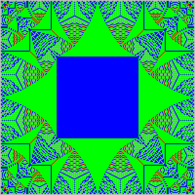
Figure 10: The identity state for the sandpile model on a 198 by 198 lattice. The color code is grey, red, blue, and green for heights 0,1,2, and 3, respectively.

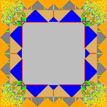
a.    b.

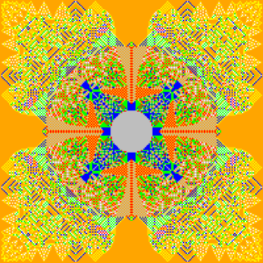
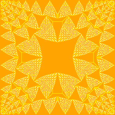
c.    d.

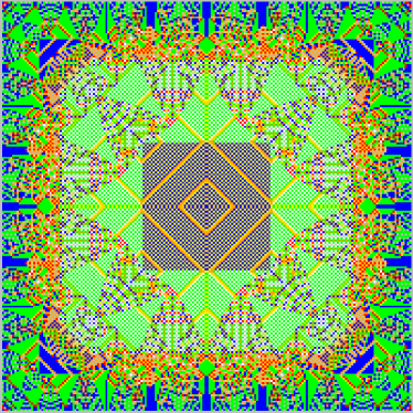
Figure 11: A procedure for constructing the identity. In parts a and b an empty table is having sand poured on from the edges. In part c the entire table is supercritical. In part d the boundaries have been opened, and the sand is running back off. The system finally relaxes the state shown in Fig. 10. In this sequence, heights are color coded as in Fig. 1, with active sites in various shades of orange. The lattice is 198 sites wide by 198 sites high.

The identity state can be constructed by taking any recursive state, say $C^{*}$ and repeatedly adding it to itself to use $|\Delta|\otimes C=I$. However, on any but the smallest lattices, $|\Delta|$ is a very large integer. A more economical scheme is given in Ref. [25]. Fig. 10 shows the identity state on a 198 by 198 lattice. Note the fractal structure, with features on many length scales.

Here I present another way to construct this state. Fig. 11a-b shows a sequence of configurations obtained by pouring sand in from the boundaries onto an initially empty table. This is accomplished by adding a temporary set of sites just outside the boundary and keeping their heights always supercritical. A variety of fractal structures emerge as the interior slowly fills up. Fig. 11c shows the final stationary state where the sand falling in from the boundaries matches that falling off from the updating. Then I revert the boundary conditions to open and allow the sand to fall back off. Fig. 11d shows an intermediate state of this procedure. When the sand finally stops falling off, I obtain the identity state as shown in Fig. 10.

Majumdar and Dhar [24] have constructed a simple “burning” algorithm to determine if a state belongs to the recursive set. For a given configuration, first add one particle to each of the edge sites and two particles to the corners. This again corresponds to imagining a large source of sand just outside the boundaries, which then tumbles one step onto the system. Then return to open boundaries and update according to the usual rules. If and only if the original state is recursive, this will generate an avalanche under which each site of the system tumbles exactly once. Also, the final state after the avalanche will be identical to the original. However, if the state is not recursive, some untumbled sites will remain. Fig. 12 shows such a process underway on the configuration of Fig. 1. Here sites which have already burned are shown in cyan, while the remaining sites in the center have not yet tumbled. The small number of sites shown in orange are the still active sites, which eventually burn the entire remaining lattice.

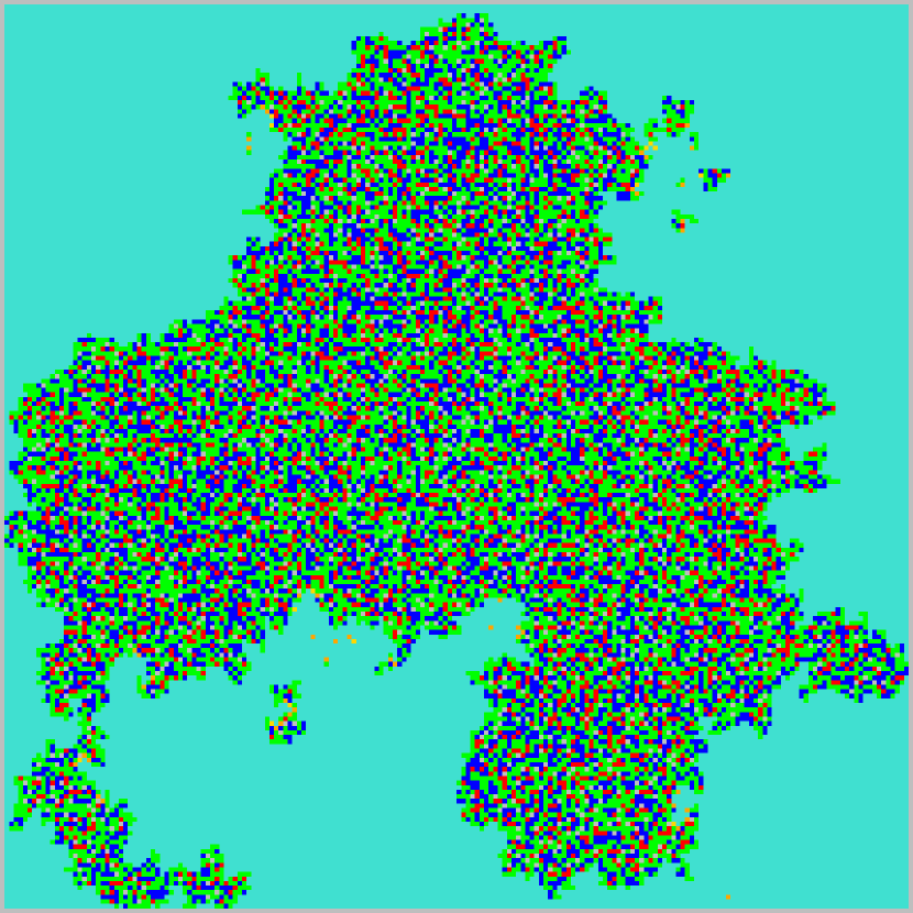
Figure 12: The burning algorithm being applied to the state in Fig. 1. Burnt sites are cyan, burning sites are orange, and the remaining sites are colored as previously. This avalanche eventually tumbles every site exactly once.

The burning algorithm provides a simple way to prove that the avalanche regions are simply connected once one is in the critical state. In a burning process, any sub-lattice of the original will have all of its sites tumbled onto from outside. This is the condition for starting a burning on the sub-lattice. Thus, if a configuration is in the critical ensemble for the whole lattice, then any extracted piece of this configuration on a subset of the original lattice is also in the critical ensemble of the extracted part. Now suppose that one constructs an avalanche with any initial addition to a state from the critical ensemble. In any subregion enclosed by this avalanche, sand will fall from the tumbling sites on its outside. Since the sub-lattice is itself in its own critical ensemble, this must induce an avalanche which, by the burning algorithm, will tumble all enclosed sites. Thus any avalanche on a state from the critical ensemble cannot leave untumbled any sites in a region isolated from the boundary, i.e. an untumbled island. This result that avalanches must be simply connected does not follow for states outside the recursive set, as can be easily demonstrated by considering a sandpile with a hole of empty sites in the middle.

9 Concluding remarks

Simple models as implemented by cellular automata provide a rich area for the study of complex phenomena. Some systems can self organize with physics at many scales, while others provide fascinating demonstrations of thermodynamic laws. I have only touched on a few issues here, leaving out many related topics such as lattice gasses, driven interfaces in random media, growth processes, and evolution. As the ease of programming and the speed of modern computers continue to rush forward, so will the fascination with such models.

References

References

- [1] P. Bak, C. Tang, and K. Wiesenfeld, Phys. Rev. Lett. 59, 381 (1987); Phys. Rev. A38, 3645 (1988).
- [2] P. Bak and M. Creutz, “Fractals and Self-organized Criticality,” chapter in Fractals in Science, A. Bunde and S. Havlin eds., pp. 26-47 (Springer-Verlag, 1994).
- [3] M. Paczuski, S. Maslov, and P. Bak, Phys. Rev. E53, 414 (1996).
- [4] K. Nagel and M. Paczuski, Phys. Rev. E51, 2909 (1995).
- [5] M. Levy, S. Solomon, and G. Ram Int. J. Mod. Phys. C7, 65 (1996).
- [6] The latest version of the xtoys package is available at the URL http://penguin.phy.bnl.gov/www/xtoys/xtoys.html.
- [7] K. Christensen, thesis, University of Aarhus.
- [8] V. Frette et al., Nature 379, 49 (1996).
- [9] S. Wolfram, editor, Theory and Applications of Cellular Automata (World Scientific, Singapore, 1986).
- [10] T. Toffoli and N. Margolus, Cellular Automata Machines (MIT Press, 1987). A good place on the web to start exploring cellular automata is the CA-FAQ at http://alife.santafe.edu/alife/topics/cas/ca-faq/ca-faq.html.
- [11] B. Bogosian, Nucl. Phys. B(Proc. Suppl.) 30, 204 (1993).
- [12] E. Berlekamp, J. Conway, and R. Guy, Winning Ways for your Mathematical Plays, volume 2, (Academic Press, ISBN 0-12-091152-3, 1982) chapter 25.
- [13] P. Callahan, http://wwwjn.inf.ethz.ch/paul/life/lifepage.html.
- [14] P. Bak, K. Chen, M. Creutz, Nature 342, 780 (1989).
- [15] M. Creutz, Nuclear Phys. B (Proc. Suppl.) 26, 252 (1992).
- [16] C. Bennett and M. Bourzutschy, Nature 350, 468 (1991).
- [17] M. Gardner, Wheels, Life, and Other Mathematical Amusements (W. H. Freeman and Company, New York, 1983).
- [18] W. Press, S. Teukolsky, W. Vetterling, and B. Flannery, Numerical Recipes in C (Cambridge University Press, 1988).
- [19] S. Clar, B. Drossel, and F. Schwabl, “Forest fires and other examples of self-organized criticality,” preprint (1996).
- [20] J.D. Murray, Mathematical Biology, pp 78-83, (Springer Verlag, 1989).
- [21] D. Dhar, Phys. Rev. Lett. 64, 1613 (1990).
- [22] D. Dhar, R. Ramaswamy, Phys. Rev. Lett. 63, 1659 (1989).
- [23] D. Dhar, S. N. Majumdar, J. Phys. A23, 4333 (1990).
- [24] S. N. Majumdar, D. Dhar, Physica A185, 129 (1992).
- [25] M. Creutz, Comp. Phys. 5, 198 (1991).
- [26] R. Anderson et al., Amer. Math. Monthly, 96, 981 (1989); A. Björner, L. Lovász, and P. Shor, Europ. J. Combinatorics 12, 283 (1991); K. Eriksson, Siam J. Discrete Math. 9, 118 (1996).
- [27] E. Goles and M. Margenstern, Int. J. of Modern Physics C7, 113 (1996).