DEVELOPMENT IN LATTICE QCD SHEP–96–33

After a brief discussion of the promise and limitations of the lattice technique, I review lattice QCD results for several quantities of phenomenological interest. These are: matrix elements for heavy-to-light meson decays, leptonic decay constants $f_{B}$ and $f_{D}$, the parameters $B_{B}$ and $B_{K}$ for neutral $B$ and $K$ meson mixing respectively, the strong coupling constant, light quark masses and the lightest scalar glueball mass.

1 Introduction

In this review I concentrate on lattice QCD results for a selection of quantities directly relevant for phenomenology, some of which were not otherwise reported at this conference. I apologise to presenters of lattice studies which I do not have space to report on here and refer the interested reader directly to the parallel session reports.

Lattice QCD is an important tool for the non-perturbative evaluation of strong interaction effects, but a wary consumer should keep in mind the main sources of error, which I will briefly mention below, when using lattice results. One beauty of the lattice approach is that these errors can be systematically investigated and reduced.

The presentation begins with form factors for $\bar{B}^{0}{\to}\pi^{+}l^{-}\bar{\nu}_{l}$, $\bar{B}^{0}{\to}\rho^{+}l^{-}\bar{\nu}_{l}$ and $\bar{B}{\to}K^{*}\gamma$. The semileptonic decays are important for determining $|V_{ub}|$; the radiative decay for $V_{ts}$ and as a window on new physics. Next follow results for the $B$ meson decay constant $f_{B}$ and mixing parameter $B_{B}$, crucial for constraining the Standard Model unitarity triangle. I then turn to the kaon mixing parameter $B_{K}$, strong coupling $\alpha_{\rm s}$ and the light quark masses, concluding with results for the lightest scalar glueball.

2 Lattice Calculations

The standard lattice approach to QCD uses a discretised finite volume region of Euclidean space-time on which the quantum field theory path integral becomes a well-defined multi-dimensional integral evaluated by Monte Carlo methods.

Current simulations use lattice spacings $a$ in the range $0.05$–$0.2\,\rm fm$, sufficient to cover a hadron of size $0.5\,\rm fm$ or greater by a few lattice points. These $a$’s correspond to energy scales of $1$–$4\,{\rm Ge\kern-1.00006ptV}$ putting the lattice ultraviolet cutoff above the scale of low energy QCD dynamics. Continuum results should be obtained in the limit $a{\to}0$: this continuum extrapolation is now feasible for many quantities. Lattices should be large enough that hadrons will comfortably fit on them. Current spatial sizes are of order $2\,\rm fm$ or so, though some practitioners advocate at least $2.5\,\rm fm$.$\!{}^{{\bf?}}$

Because the QCD action is quadratic in the quark fields, matrix elements of quarks can be evaluated using quark propagators in the gluon background together with the gluon-field-dependent determinant of the fermion operator. The determinant is extremely demanding to calculate so it is often set to its average value in the gauge field background—the quenched approximation—which corresponds to neglecting internal quark loops. In practice, much of the effect of internal loops is to change the running of the coupling constant and this can be compensated by changing the value of $\beta$, the bare coupling which is input. Quenching is one of the systematic effects causing disagreement between lattice spacings determined from different physical quantities.

Calculating quark propagators means inverting the fermion operator. This is very slow for realistic light quarks, so a range of masses around the strange mass is simulated and then a ‘chiral extrapolation’ made to realistic values. For heavy quark masses $m$, the inversion is fast but for large $ma$ discretisation errors are large. Hence, $B$ physics results using relativistic fermion actions typically involve an extrapolation from results at masses close to the charm scale. An alternative is to use static or nonrelativistic (NRQCD) lattice actions. In the static case the quark mass is treated analytically, outside the simulation, and results are obtained in a systematic expansion around the infinite mass limit. NRQCD actions work well for quarks around the $b$ mass and above, but begin to fail as one approaches the $c$ mass. Actions are also used which interpolate between the static and relativistic extremes.$\!{}^{{\bf?}}$

Lattice calculations provide matrix elements of bare operators defined with the lattice regularisation, but results are needed for matrix elements in a continuum scheme, like $\overline{\rm MS}$. A continuum operator typically matches onto a set of lattice operators,

$${\cal O}_{i}^{\rm cont}(\mu)=Z_{ij}(\mu,a){\cal O}_{j}^{\rm latt}(a),$$

where the renormalisation constants $Z_{ij}$ can be calculated perturbatively. Lattice perturbation theory using the bare coupling $g_{0}^{2}=6/\beta$ is notoriously badly-behaved, however. $\!{}^{{\bf?}}$ Abandoning $g_{0}^{2}$ in favour of a continuum-like definition leads to better behaviour, but nonperturbative methods are being developed and used (some are mentioned below).$\!{}^{{\bf?}}$ This looks to be the way of the future.

Lattice gluon actions have discretisation errors beginning at $O(a^{2})$. The simplest, Wilson, fermion action, a latticised relativistic Dirac action, has errors beginning at $O(a)$. One can simply accept the $O(a)$ errors and let the $a{\to}0$ extrapolation remove them. However, removing or reducing the $O(a)$ errors allows simulations at coarser lattice spacings and makes the continuum extrapolation less severe. This ‘improvement’ of lattice actions is currently a very active subject. The Sheikholeslami-Wohlert $\!{}^{{\bf?}}$ (SW or ‘clover’) action removes $O(a)$ errors at tree level, so the first corrections are $O(\alpha_{\rm s}a)$. The SW action contains one extra term compared to the Wilson action. By tuning the coefficient of this term one can reduce or even remove all $O(a)$ errors in physical quantities (one has to improve operators used in matrix element calculations also). Partial removal using ‘tadpole-improvement’ $\!{}^{{\bf?}}$ is being widely applied, but an ambitious program by the ALPHA collaboration $\!{}^{{\bf?},{\bf?}}$ aims for complete removal.

3 Semileptonic and Radiative Heavy-to-light Decays

Lattice form factor calculations are crucial here: the overall normalisation at the zero recoil point $\omega=v{\cdot}v^{\prime}=1$ is not fixed by heavy quark symmetry as it is for a heavy-to-heavy transition. Here $v$ and $v^{\prime}$ are the four-velocities of the $B$ meson of mass $M$ and the meson of mass $m$ it decays into, respectively. The squared momentum transfer to the leptons or photon is $q^{2}=M^{2}+m^{2}-2Mm\omega$.

$q^{2}\!/\!\,{\rm Ge\kern-1.00006ptV}^{2}$ $M\!/\!\,{\rm Ge\kern-1.00006ptV}$ $D$ $B$

Figure 1: $q^{2}$ range for heavy-to-light decays as a function of the decaying heavy meson mass. Lines of constant $\omega$ are shown. The light final state mass is taken to be $850\,{\rm Me\kern-1.00006ptV}$, typical of lattice pseudoscalar or vector meson masses before chiral extrapolation.

Relativistic quark calculations use heavy quark masses around the charm mass. The initial heavy meson is given $0$ or $1$ lattice units of three-momentum, while the light final meson can generally be given up to two lattice units of spatial momentum, allowing $q^{2}$ to be varied from $q^{2}_{\rm max}=(M{-}m)^{2}$ (where $\omega=1$) down to $q^{2}<0$ at the $D$ scale. Heavy quark symmetry determines the $M$ dependence of the form factors at fixed $\omega$, enabling an extrapolation to the $B$ scale. Fig. 1 shows that scaling in $M$ at fixed $\omega$ sweeps all the measured points to a region near $q^{2}_{\rm max}$ for $B$ decays. The problem is then to extrapolate back down to $q^{2}=0$. This is particularly acute for the radiative decay $\bar{B}{\to}K^{*}\gamma$ where only the form factors at $q^{2}=0$ contribute. Even if a static, non-relativistic or other modified action is used for the heavy quark, the restriction on usable three-momenta on current lattices, caused by momentum-dependent errors and increasing statistical uncertainty, ensures that form factor values are obtained only near $q^{2}_{\rm max}$.$\!{}^{{\bf?}}$

Some assistance is provided by ensuring that any model $q^{2}$ dependences respect heavy quark symmetry and constraints relating form factors at $q^{2}=0$. For example, $f^{+}$ and $f^{0}$ for $B\to\pi$ are related at $q^{2}=0$ and consistency can be achieved by fitting $f^{+}$ to a dipole [pole] form and $f^{0}$ to a pole [constant] form. Heavy quark symmetry and light flavour $SU(3)$ symmetry relate the $\bar{B}^{0}{\to}\rho^{+}l^{-}\bar{\nu}_{l}$ and $\bar{B}{\to}K^{*}\gamma$ form factors. Models can further relate these to form factors for $\bar{B}^{0}{\to}\pi^{+}l^{-}\bar{\nu}_{l}$. An overall fit might then be used. However, it is clearly desirable to avoid models entirely.

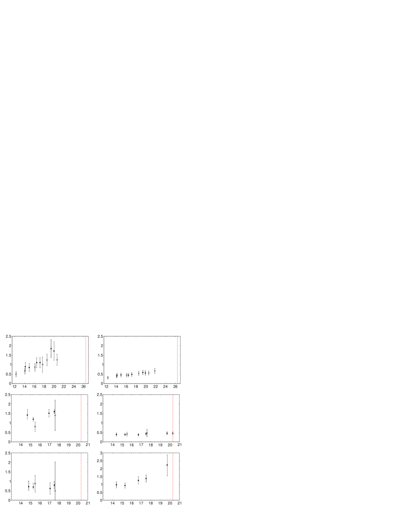
$q^{2}/\!\,{\rm Ge\kern-1.00006ptV}^{2}$ $f^{+}$ $V$ $A_{2}$ $f^{0}$ $A_{1}$ $A_{0}$

Figure 2: Lattice measurements of the form factors for $\bar{B}^{0}{\to}\pi^{+}l^{-}\bar{\nu}_{l}$ and $\bar{B}^{0}{\to}\rho^{+}l^{-}\bar{\nu}_{l}$. Points are from ELC $\!{}^{{\bf?}}$ ($\equiv$), APE $\!{}^{{\bf?},{\bf?}}$ ($=$), UKQCD $\!{}^{{\bf?}}$ ($\bullet$) and FNAL $\!{}^{{\bf?},{\bf?}}$ ($\times$, preliminary). Systematic errors have been added $\!{}^{{\bf?}}$ to the UKQCD and FNAL points. The vertical dashed lines show $q^{2}_{\rm max}$.

3.1 Semileptonic $B\to\pi$

Lattice results $\!{}^{{\bf?},{\bf?},{\bf?},{\bf?}}$ for the $\bar{B}^{0}{\to}\pi^{+}l^{-}\bar{\nu}_{l}$ form factors, $f^{+}$ and $f^{0}$, are plotted in Fig. 2 (further results $\!{}^{{\bf?},{\bf?}}$ at $q^{2}=0$ only are not displayed).

For massless leptons, the decay rate is determined by $f^{+}$ alone. However, the constraint $f^{+}(0)=f^{0}(0)$ (with suitable conventions) makes lattice measurements of both form factors useful. One procedure uses dispersive constraints, obtained by combining dispersion relations with unitarity, analyticity, crossing symmetry and perturbative QCD, to obtain model independent bounds. Lellouch $\!{}^{{\bf?},{\bf?}}$ has shown how to incorporate the $f^{+}(0)=f^{0}(0)$ condition together with imperfectly known values of the form factors, typical of lattice results with errors, to obtain families of bounds with varying confidence levels. A set of such bounds is shown in Fig. 3 together with the UKQCD $\!{}^{{\bf?}}$ lattice measurements used to obtain them. In the figure, $f^{0}$ and $f^{+}$ are plotted back-to-back, showing the effect of imposing the constraint at $q^{2}=0$.

In Table 1 the bounds have been used to give ranges of values for the decay rate $\Gamma(\bar{B}^{0}{\to}\pi^{+}l^{-}\bar{\nu}_{l})$ in units of $|V_{ub}|^{2}\,{\rm ps}^{-1}$ together with values for the form factor $f^{+}$ at $q^{2}=0$. When combined with the experimental result for the decay rate, one can extract $|V_{ub}|$ with about 35% theoretical error. Although not very precise, this result relies only on lattice calculations of matrix elements and heavy quark symmetry, together with perturbative QCD and analyticity properties in applying the dispersive constraints. There is no model dependence. Improved lattice results can be used as input for the bounds once they become available.

Also shown in Table 1, for comparison, are values obtained from lattice calculations where assumed $q^{2}$ dependences have been imposed. For ELC $\!{}^{{\bf?}}$ and APE,$\!{}^{{\bf?}}$ one value of $f^{+}$ has been used, at the given value of $q^{2}$, fitted to a single pole form with pole mass $m_{\rm p}$. The UKQCD result $\!{}^{{\bf?}}$ is obtained from a combined dipole/pole fit to all measured $f^{+}$/$f^{0}$ points. Note that the UKQCD points have statistical errors only and have not been chirally extrapolated—they correspond to a pion mass of around $800\,{\rm Me\kern-1.00006ptV}$ (a similar caveat applies for the FNAL $\!{}^{{\bf?},{\bf?}}$ results for $f^{+}$ and $f^{0}$). The results given $\!{}^{{\bf?}}$ have used these values as though they applied to the physical pion. In obtaining bounds based on these points, Lellouch $\!{}^{{\bf?}}$ added a conservatively estimated systematic error including terms to account for the chiral extrapolation (this error has been added to the UKQCD and FNAL points plotted in Fig. 2).

Table 1: $\bar{B}^{0}{\to}\pi^{+}l^{-}\bar{\nu}_{l}$ results from dispersive constraints applied to lattice data,$\!{}^{{\bf?}}$ together with results obtained using ansätze for the form factor $f^{+}$. The decay rates are values for $\Gamma(\bar{B}^{0}{\to}\pi^{+}l^{-}\bar{\nu}_{l})/|V_{ub}|^{2}{\rm ps}^{-1}$

	Rate	$f^{+}(0)$
Dispersive	$2.4$–$28$	$-0.26$–$0.92$	95% CL
Constraint $\!{}^{{\bf?}}$	$3.6$–$17$	$0.00$–$0.68$	70% CL
	$4.8$–$10$	$0.18$–$0.49$	30% CL
ELC $\!{}^{{\bf?}}$	$9\pm 6$	0.10–0.49
$q^{2}{\simeq}18\,{\rm Ge\kern-1.00006ptV}^{2}$, pole fit, $m_{\rm p}{=}5.29(1)\,{\rm Ge\kern-1.00006ptV}$
APE $\!{}^{{\bf?}}$	$8\pm 4$	0.23–0.43
$q^{2}{\simeq}20.4\,{\rm Ge\kern-1.00006ptV}^{2}$, pole fit, $m_{\rm p}{=}5.32(1)\,{\rm Ge\kern-1.00006ptV}$
UKQCD $\!{}^{{\bf?},{\bf?}}$	$7\pm 1$	0.21–0.27
dipole/pole fit to $f^{+}$/$f^{0}$

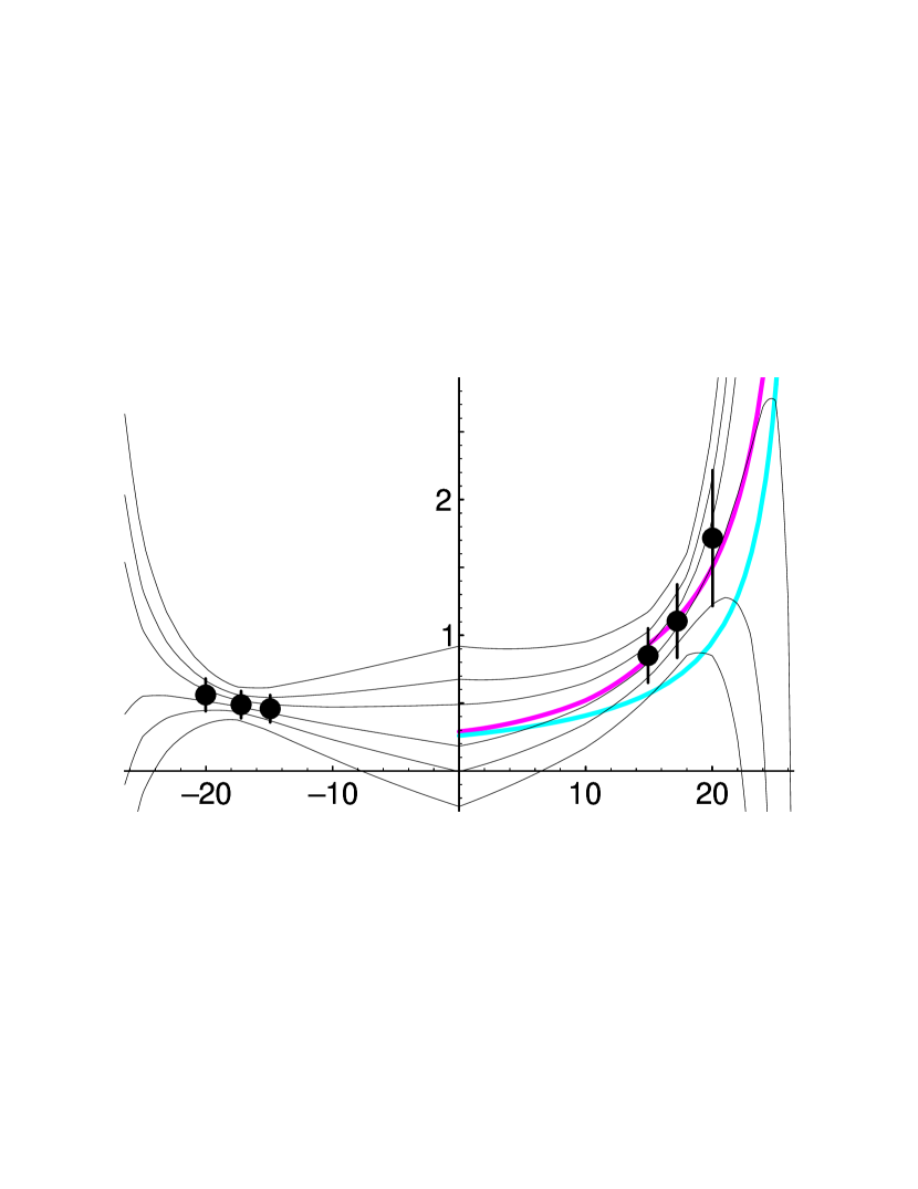
$f^{+}(q^{2})$ $f^{0}(|q^{2}|)$ $q^{2}/\,{\rm Ge\kern-1.00006ptV}^{2}$

Figure 3: Bounds on $f^{+}$ and $f^{0}$ for $\bar{B}^{0}{\to}\pi^{+}l^{-}\bar{\nu}_{l}$ from dispersive constraints.$\!{}^{{\bf?}}$ The data points are from UKQCD,$\!{}^{{\bf?}}$ with added systematic errors. The pairs of fine curves are, outermost to innermost, 95%, 70% and 30% bounds. The upper and lower shaded curves are light-cone $\!{}^{{\bf?}}$ and three-point $\!{}^{{\bf?}}$ sum rule results respectively.

Chiral extrapolations are severe for the $B\to\pi$ matrix elements. As the pion mass approaches its physical value the $B^{*}$-pole and the beginning of the $B\pi$ continuum approach $q^{2}_{\rm max}$ from above and the form factors may vary rapidly with the pion mass near $q^{2}_{\rm max}$. This is not a problem for $B\to\rho$ so lattice calculations of semileptonic $B\to\rho$ decay are currently most reliable and I now turn to them.

3.2 Semileptonic $B\to\rho$

To avoid models for the $q^{2}$ dependence of the form factors, we use the lattice results directly. The lattice can give the differential decay rate $d\Gamma/dq^{2}$, or the partially integrated rate, in a $q^{2}$ region near $q^{2}_{\rm max}$ up to the unknown factor $|V_{ub}|^{2}$. For example, UKQCD $\!{}^{{\bf?}}$ parametrised the differential decay rate near $q^{2}_{\rm max}$ by,

$${d\Gamma\over dq^{2}}={\rm const}|V_{ub}|^{2}q^{2}\lambda^{1/2}a^{2}\big{(}1+b[q^{2}{-}q^{2}_{\rm max}]\big{)},$$ (1)

where $\lambda$ is the usual phase space factor and $a$ and $b$ are constants. The constant $a$ plays the role of the Isgur-Wise function evaluated at $\omega=1$ for heavy-to-heavy transitions, but in this case there is no symmetry to determine its value.

For massless leptons, the differential decay rate depends on the $V$, $A_{1}$ and $A_{2}$ form factors, but $A_{1}$ is the dominant contribution near $q^{2}_{\rm max}$ and is also the best measured on the lattice, as shown in Fig. 2. UKQCD performed a fit to the parametrisation in Eq. (1) to find,$\!{}^{{\bf?}}$

$$a=4.6{}^{+0.3}_{-0.4}\pm 0.6\,{\rm Ge\kern-1.00006ptV}.$$

Discounting experimental errors, this result will allow determination of $|V_{ub}|$ with a theoretical uncertainty of 10% statistical and 12% systematic. CLEO are beginning to extract the differential decay distributions.$\!{}^{{\bf?}}$

The UKQCD results for $V$, $A_{1}$ and $A_{2}$ agree very well with a light cone sum rule (LCSR) calculation of Ball and Braun.$\!{}^{{\bf?}}$ More interestingly, LCSR calculations predict that all the form factors for heavy-to-light decays have the following heavy mass dependence at $q^{2}=0$: $\!{}^{{\bf?},{\bf?}}$

$$f(0)={1\over M^{3/2}}(a_{0}+a_{1}/M+a_{2}/M^{2}+\cdots).$$ (2)

The leading $M$ dependence comprises $\sqrt{M}$ from the heavy state normalisation together with the behaviour of the leading twist light cone wavefunction. For $A_{1}(0)$ the LCSR result is $\!{}^{{\bf?}}$ $A_{1}(0)\simeq 0.26$. UKQCD fitted the heavy mass dependence of $A_{1}(0)$ to the form in Eq. (2) and found $\!{}^{{\bf?}}$

$$A_{1}(0)=\cases{0.18\pm 0.02&$a_{0}$ and $a_{1}\neq 0$\cr 0.22{}^{+0.04}_{-0.03}&$a_{0}$, $a_{1}$ and $a_{2}\neq 0$\cr}$$

Pole fits for $A_{1}$ have leading $M^{-3/2}$ behaviour at $q^{2}=0$, so we can also compare with other lattice results:

$$A_{1}(0)=\cases{0.22\pm 0.05&ELC \immediate{$\!{}^{{\bf?}}$}\cr 0.24\pm 0.12&APE \immediate{$\!{}^{{\bf?}}$}\cr 0.27{}^{+7}_{-4}&UKQCD \immediate{$\!{}^{{\bf?}}$}\cr}$$

3.3 Rare radiative $B\to K^{*}\gamma$

This decay was discussed in some detail by A. Soni at Lattice 95 $\!{}^{{\bf?}}$ so my comments will be brief. Table 2 summarises available lattice results, all from quenched simulations, for the matrix element

$$\langle K^{*}(k,\eta)|\overline{s}\sigma_{\mu\nu}q^{\nu}b_{R}|B(p)\rangle$$ (3)

which is parameterised by three form factors, $T_{i}$, $i=1,2,3$. For the decay rate, the related values $T_{1}(0)$ and $T_{2}(0)$ are needed. Suitably defined, they are equal, so the table lists a single value $T(0)$, together with the directly measured $T_{2}(q^{2}_{\rm max})$. The results are classified by the leading $M$ dependence of the form factor at $q^{2}=0$ which is governed by the model used for the $q^{2}$ dependence. Dipole/pole forms for $T_{1}$/$T_{2}$ give $M^{-3/2}$ behaviour and pole/constant forms give $M^{-1/2}$. The results agree when the same assumptions are made. All groups find that $T_{2}$ has much less $q^{2}$ dependence than $T_{1}$, but the overall forms cannot be decided, so a phenomenological prediction is elusive.

Table 2: Lattice results for $\bar{B}{\to}K^{*}\gamma$.

	$T(0)$
	$M^{-3/2}$	$M^{-1/2}$	$T_{2}(q^{2}_{\rm max})$
BHS $\!{}^{{\bf?}}$	0.10(3)		0.33(7)
LANL $\!{}^{{\bf?}}$	0.09(1)	0.24(1)
APE $\!{}^{{\bf?}}$	0.09(1)	0.23(3)	0.23(3)
UKQCD $\!{}^{{\bf?}}$	0.15$(^{7}_{6})$	0.26$(^{2}_{1})$	0.27$(^{2}_{1})$
BHS $\!{}^{{\bf?}}$			0.30(3)

Additional long distance contributions may not be negligible so the matrix element of Eq. (3) may not give the true decay rate.$\!{}^{{\bf?},{\bf?},{\bf?}}$ Once the $q^{2}$ dependence of the form factors is known, lattice calculations of the ratio $R_{K^{*}}=\Gamma(\bar{B}{\to}K^{*}\gamma)/\Gamma(b\to s\gamma)$ can be compared to the experimental result to test for long distance effects.

4 Leptonic Decay Constants $f_{B}$ and $f_{D}$

Table 3: Values and ratios of leptonic decay constants of pseudoscalar mesons from recent continuum extrapolations by MILC $\!{}^{{\bf?}}$ and JLQCD $\!{}^{{\bf?}}$. Statistical and systematic errors have been combined in quadrature. The MILC results include a systematic error for quenching. The bottom row contains summary values based on global data.$\!{}^{{\bf?},{\bf?},{\bf?},{\bf?}}$

	$f_{B}/\,{\rm Me\kern-1.00006ptV}$	$f_{B_{s}}/\,{\rm Me\kern-1.00006ptV}$	$f_{B_{s}}/f_{B}$	$f_{D}/\,{\rm Me\kern-1.00006ptV}$	$f_{D_{s}}/\,{\rm Me\kern-1.00006ptV}$	$f_{D_{s}}/f_{D}$
MILC $\!{}^{{\bf?}}$	166(33)	181(41)	1.10(10)	196(18)	211(28)	1.09(7)
JLQCD $\!{}^{{\bf?}}$	179$(^{11}_{33})$	197$(^{\phantom{0}7}_{36})$		202$(^{25}_{14})$	216$(^{23}_{16})$
Summary	175(25)	200(25)	1.15(5)	205(15)	235(15)	1.15(5)

The leptonic decay constant of a pseudoscalar meson $P$ is defined by the axial current matrix element

$$\left\langle 0\right|A_{\mu}(0)\left|P(p)\right\rangle=if_{P}p_{\mu}.$$

On the lattice one calculates a dimensionless quantity $Z_{L}$, from which $f_{P}$ is obtained via

$$f_{P}\sqrt{M_{p}/2}=Z^{\rm ren}Z_{L}a^{-3/2}$$

where $Z^{\rm ren}$ is the renormalisation constant required to match to the continuum and $a$ is the lattice spacing.

Two collaborations have new values, shown in table 3, for $f_{B}$ and $f_{D}$ obtained from continuum extrapolations of quenched results at several lattice spacings. JLQCD $\!{}^{{\bf?}}$ study different prescriptions for reducing the $O(ma)$ discretisation errors associated with heavy quarks and aim to show that all results converge in the continuum limit. Their error is statistical combined with an error from the spread over prescriptions.

MILC $\!{}^{{\bf?}}$ simulate a range of heavy quark masses plus a static (infinite mass) quark, giving meson masses straddling $m_{D}$ and allowing an interpolation to $m_{B}$. Their (preliminary) results give errors from: (i) statistics, (ii) systematics within the quenched approximation and (iii) unquenching—they have dynamical fermion results but do not yet perform a continuum extrapolation with them. Their results suggest that unquenching will raise the value of the decay constants. This agrees with an estimate,$\!{}^{{\bf?},{\bf?}}$ using the difference between chiral loop contributions in quenched and unquenched QCD, that $f_{B_{s}}$ in full QCD is increased by 20% over its quenched value. Calculations of $f_{B}$ in the static limit extrapolated from negative numbers of flavours $\!{}^{{\bf?}}$ also suggest an increase of about 20%.

The SGO collaboration $\!{}^{{\bf?},{\bf?}}$ is calculating $f_{B}$ using a lattice NRQCD action (and heavy-light axial current) corrected to $O(1/M)$ where $M$ is the heavy quark mass. However, the renormalisation constants required to match onto full QCD are not yet available, so I will not quote results for the decay constant.

The last row of table 3 summarises $\!{}^{{\bf?}}$ global results for $B$ and $D$ meson decay constants, following the compilation by G. Martinelli. $\!{}^{{\bf?},{\bf?},{\bf?}}$

5 $B$–$\bar{B}$ Mixing Parameter

Recent lattice calculations of the $B$ meson mixing parameter $B_{B}(\mu)$, defined analogously to the kaon mixing parameter $B_{K}$ in Eq. 4 below, have been made both for relativistic quarks $\!{}^{{\bf?},{\bf?}}$ and in the static limit.$\!{}^{{\bf?},{\bf?},{\bf?}}$ The latest static results $\!{}^{{\bf?},{\bf?}}$ use new calculations of the full-theory/static-theory matching incorporating previously omitted contributions.$\!{}^{{\bf?},{\bf?}}$ Since $B_{B}(\mu)$ is scale-dependent it is conventional to quote a renormalisation group invariant (RGI) quantity, $\hat{B}_{B}$. At one loop $\hat{B}_{B}=\alpha_{\rm s}(\mu)^{-2/\beta_{0}}B_{B}(\mu)$, but the two-loop relation is commonly used.$\!{}^{{\bf?},{\bf?}}$

Calculations with relativistic quarks show no obvious lattice spacing dependence and cluster around a value of $\hat{B}_{B}=1.3(1)$ [with a weighted average of $1.31(3)$, quoted in Warsaw] for the one-loop $B$ parameter,$\!{}^{{\bf?},{\bf?}}$ or $\hat{B}_{B}=1.4(1)$ using the two-loop formula.$\!{}^{{\bf?}}$ Allowing for uncertainty in the continuum extrapolation, I quote the two-loop $\hat{B}_{B}=1.4(1)$ as the quenched lattice result.

The static results differ for calculations using Wilson $\!{}^{{\bf?}}$ or SW $\!{}^{{\bf?},{\bf?}}$ light quarks. The Kentucky group $\!{}^{{\bf?}}$ (Wilson) find $\hat{B}_{B}=1.40(6)$ for the one-loop RGI quantity, rising to $1.50(6)$ for the two-loop case. The APE two-loop result $\!{}^{{\bf?}}$ (SW) is $\hat{B}_{B}=1.08(6)(8)$. The dominant uncertainty is from higher order terms in the perturbative matching to continuum QCD. Nonperturbative renormalisation will be crucial to reduce systematic errors.$\!{}^{{\bf?},{\bf?}}$

The relevant quantity for $B$–$\bar{B}$ mixing is $\xi_{B}^{2}=f_{B}^{2}\hat{B}_{B}$. Taking the two-loop relativistic quark result for $\hat{B}_{B}$ with $f_{B}=175(25)\,{\rm Me\kern-1.00006ptV}$ from table 3 gives $\xi_{B}=207(30)\,{\rm Me\kern-1.00006ptV}$ as the current lattice estimate.$\!{}^{{\bf?}}$ This quantity can also be extracted directly from the $\Delta B{=}2$ matrix element, $M=8f_{B}^{2}B_{B}m_{B}^{2}/3$. To avoid uncertainties from setting the scale, it is convenient to determine the ratio $\!{}^{{\bf?}}$

$$r_{sd}={f_{B_{s}}^{2}B_{B_{s}}m_{B_{s}}^{2}\over f_{B}^{2}B_{B}m_{B}^{2}}$$

For relativistic quarks a direct extraction gives $r_{sd}=1.54(13)(32)$. Previously, $r_{sd}$ has been evaluated from separate results for the decay constant and $B$ parameter ratios. Combining $f_{B_{s}}/f_{B}=1.15(5)$ from table 3 with $B_{B_{s}}/B_{B}=1.01(4)$ $\!{}^{{\bf?}}$ and $m_{B_{s}}/m_{B}=1.017$ gives $r_{sd}=1.38(13)$. In the static case, APE $\!{}^{{\bf?}}$ find $r_{sd}=1.35(5)$ by the direct method, or $r_{sd}=1.43(7)$ from combining $f_{B_{s}}/f_{B}=1.17(3)$ and $B_{B_{s}}/B_{B}=1.01(1)$ measured on the same gauge configurations. The results of the two methods are quite consistent, but future calculations should improve on the precision of $r_{sd}$ obtained directly.

The above results are from quenched calculations. Unquenching is expected to increase $f_{B_{s}}/f_{B}$ by about 10% ($0.16$ from a chiral loop estimate $\!{}^{{\bf?},{\bf?}}$). For $B_{B_{s}}/B_{B}$, numerical evidence suggests a small increase on two-flavour dynamical configurations $\!{}^{{\bf?}}$ but the chiral loop estimate $\!{}^{{\bf?},{\bf?}}$ is for a decrease of $-0.04$ in the ratio.

6 Kaon $B$-Parameter $B_{K}$

The parameter $B_{K}$ is defined by

$$B_{K}(\mu)={\langle\bar{K}^{0}|\bar{s}\gamma_{\mu}Ld\bar{s}\gamma^{\mu}Ld|K^{0}\rangle\over 8\langle\bar{K}^{0}|\bar{s}\gamma_{\mu}Ld\left|0\right\rangle\langle 0|\bar{s}\gamma^{\mu}Ld\left|K\right\rangle\!/3},$$ (4)

where $L=1{-}\gamma_{5}$. It is a scale dependent quantity for which lattice results are most often quoted after translation to the value in $\overline{\rm MS}$ using naive dimensional regularisation (NDR) at a scale $\mu=2\,{\rm Ge\kern-1.00006ptV}$. I will follow this practice while discussing the lattice results and convert at the end to the renormalisation group invariant parameter $\hat{B}_{K}$ normally used in phenomenology. At next-to-leading order, $\hat{B}_{K}$ is given by,

$${\hat{B}_{K}\over B_{K}(\mu)}=\alpha_{\rm s}(\mu)^{{-\gamma_{0}\over 2\beta_{0}}}\Big{(}1+{\alpha_{\rm s}(\mu)\over 4\pi}{(\beta_{1}\gamma_{0}-\beta_{0}\gamma_{1})\over 2\beta_{0}^{2}}\Big{)},$$

where $\beta_{0,1}$ and $\gamma_{0,1}$ are the first two coefficients of the beta function and anomalous dimension, respectively.$\!{}^{{\bf?},{\bf?}}$

Systematic errors in $B_{K}$ calculations are being carefully explored. Calculations using staggered fermions (an alternative formulation of relativistic lattice fermions) are statistically more precise, but Wilson fermion results are rapidly improving. Here I summarise the current situation. For more details see the report by S. Sharpe from Lattice 96.$\!{}^{{\bf?}}$

6.1 Staggered $B_{K}$

Discretisation errors for $B_{K}$ using staggered fermions are known to be $O(a^{2})$.$\!{}^{{\bf?}}$ The first calculation $\!{}^{{\bf?}}$ performed with a range of lattice spacings $a$ therefore used a quadratic extrapolation in $a$ and found $B_{K}^{\rm NDR}(2\,{\rm Ge\kern-1.00006ptV})=0.616(20)(27)$ for the quenched result. The data itself, however, could not distinguish linear and quadratic $a$ dependence. New results from the JLQCD collaboration $\!{}^{{\bf?},{\bf?}}$ are shown in Fig. 4. Their data fits better to a linear than a quadratic dependence on $a$. The argument for $O(a^{2})$ corrections has been checked,$\!{}^{{\bf?},{\bf?},{\bf?}}$ however, so results are quoted for a quadratic fit.$\!{}^{{\bf?}}$ Future calculations at smaller $a$ should confirm the leading $a^{2}$ dependence. A continuum-extrapolated quenched result has also been given by a group from OSU.$\!{}^{{\bf?}}$ The new results are ($n_{f}$ is the number of dynamical flavours):

$$B_{K}^{\rm NDR}(2\,{\rm Ge\kern-1.00006ptV})_{{a\to 0\atop n_{f}=0}}=\cases{0.587(7)(17)&JLQCD\cr 0.573(15)&OSU\cr}$$ (5)

I will take these as the best quenched lattice estimates of $B_{K}$.

Figure 4: JLQCD results $\!{}^{{\bf?}}$ for $B_{K}^{\rm NDR}(2\,{\rm Ge\kern-1.00006ptV})$ as a function of $m_{\rho}a$, with a quadratic fit to four leftmost data points (solid) and a linear fit to five leftmost data points (dashed). “Non-inv” and “Inv” refer to two possible discretisations of the lattice operators.

Two issues need addressing to relate the results in Eq. (5) to $B_{K}$ for full QCD. One is the inclusion of dynamical quarks. The second is to allow $m_{s}\neq m_{d}$, since the calculations above have a kaon composed from degenerate quarks.

Important progress in unquenching $B_{K}$ has been made by the OSU group,$\!{}^{{\bf?}}$ who find a statistically significant increase in $B_{K}$ (earlier studies suggested a small decrease $\!{}^{{\bf?}}$),

$${B_{K}^{\rm NDR}(2\,{\rm Ge\kern-1.00006ptV})^{n_{f}=3}\over B_{K}^{\rm NDR}(2\,{\rm Ge\kern-1.00006ptV})^{n_{f}=0}}=1.05(2).$$ (6)

They calculated with $n_{f}=0,2,4$ for fixed lattice spacing $a=2\,{\rm Ge\kern-1.00006ptV}$. Sharpe $\!{}^{{\bf?}}$ gives a more conservative estimate for the ratio as $1.05(15)$ after allowing for the extrapolation to $a{=}0$.

To calculate $B_{K}$ with physical mass non-degenerate quarks requires fermions with very small masses and will therefore be difficult. However, chiral perturbation theory fixes the quark mass dependence of $B_{K}$, providing a way to determine the non-degeneracy correction.$\!{}^{{\bf?},{\bf?}}$ The calculation has yet to be done, so Sharpe $\!{}^{{\bf?}}$ estimates,

$$B_{K}^{\rm nondegen}=1.05(5)\,B_{K}^{\rm degen}.$$ (7)

Combining the staggered fermion results in Eq. (5) with the unquenching and nondegeneracy corrections in Eqs. (6) and (7) leads to the final estimate:

$$B_{K}^{\rm NDR}(2\,{\rm Ge\kern-1.00006ptV})=0.64(2)(10).$$ (8)

The first error is that in the quenched value. The second is the larger 15% unquenching error combined in quadrature with the 5% error for nondegeneracy. Since Eq. (8) incorporates estimates of systematic effects in the central value, an alternative statement is $B_{K}^{\rm NDR}(2\,{\rm Ge\kern-1.00006ptV})=0.58(2)(9)$, where the central value is the quenched result, noting that unquenching and nondegeneracy can raise the value by 10%. Converting the result in Eq. (8) to $\hat{B}_{K}$ using $\alpha_{\rm s}(2\,{\rm Ge\kern-1.00006ptV})=0.3$ and three flavours gives 

$$\hat{B}_{K}=0.87(3)(14).$$

6.2 Wilson $B_{K}$

Calculations of $B_{K}$ using Wilson and SW fermions have to deal with the explicit breaking of chiral symmetry by the fermion action. This means that the continuum operator of interest mixes with four other dimension six lattice operators:

$${\cal O}^{\rm cont}=Z\big{(}{\cal O}^{\rm latt}+\sum_{i=1}^{4}z_{i}{\cal O}_{i}\big{)}+O(a).$$

The constants $Z$ and $z_{i}$ have to be determined so that lattice and continuum matrix elements agree to $O(a)$. A general four-fermion operator has the chiral expansion

$$\langle\bar{K}|{\cal O}\left|K\right\rangle=\alpha+\beta m_{K}^{2}+\delta_{1}m_{K}^{4}+$$

$$p_{\bar{K}}\mathord{\cdot}p_{K}(\gamma+\delta_{2}m_{K}^{2}+\delta_{3}p_{\bar{K}}\mathord{\cdot}p_{K})+\cdots.$$

For the continuum operator used to determine $B_{K}$, chiral symmetry demands that $\alpha=\beta=\delta_{1}=0$. The vanishing of these momentum-independent lattice artifacts can be used to test that the $z_{i}$ are correct.

Various methods have been applied to determine the $z_{i}$ and $Z$. One loop perturbation theory gives incorrect chiral behaviour. One can adjust the $z_{i}$ by hand to restore the correct behaviour $\!{}^{{\bf?},{\bf?}}$ or calculate with varying momenta to isolate and discard the artifacts.$\!{}^{{\bf?},{\bf?}}$ A better procedure is to calculate $Z$ and the $z_{i}$ nonperturbatively. The Rome group demand that quark matrix elements satisfy continuum normalisation conditions,$\!{}^{{\bf?},{\bf?},{\bf?}}$ while JLQCD $\!{}^{{\bf?}}$ impose chiral Ward identities on quark matrix elements to determine the $z_{i}$, together with a continuum normalisation step to fix $Z$. Both groups find that the matrix element of ${\cal O}^{\rm cont}$ is obtained with the correct chiral behaviour. The errors are currently larger than for staggered fermions, principally because of the need to calculate several constants $z_{i}$.

JLQCD $\!{}^{{\bf?}}$ find that the continuum extrapolation is best done for a quantity differing from $B_{K}$ by lattice artifacts which vanish as $a{\to}0$. Extrapolating from results at three different $a$ values they find $B_{K}^{\rm NDR}(2\,{\rm Ge\kern-1.00006ptV})^{n_{f}=0}_{a\to 0}=0.59(8)$, in excellent agreement with the staggered results in Eq. (5).

7 Strong Coupling $\alpha_{\rm s}$

Determinations of $\alpha_{\rm s}$ from Lattice QCD are done in three steps: (i) define and measure some $\alpha_{\rm s}^{\rm latt}$, (ii) determine the lattice spacing $a$, to set the scale at which $\alpha_{\rm s}^{\rm latt}$ takes its measured value, and (iii) convert to $\alpha_{\rm\overline{MS}}$. Step (i) is necessary because the bare lattice coupling, determined from the simulation parameter $\beta=6/g^{2}$, is rather small and has a badly-behaved perturbation theory. One must instead use a physical definition for $\alpha_{\rm s}^{\rm latt}$. Steps (ii) and (iii) are the major source of uncertainty. Here I will give an update and refer the reader to recent reviews for more details.$\!{}^{{\bf?},{\bf?},{\bf?}}$ New results are available $\!{}^{{\bf?}}$ from the NRQCD collaboration and a Fermilab-SCRI group, both using quarkonium level splittings to fix the lattice spacing. Other lattice methods of determining $\alpha_{\rm s}$ are being developed. These include studying the three gluon vertex $\!{}^{{\bf?}}$ and a program by the ALPHA collaboration using the Schrödinger Functional method, outlined by S. Sint at this conference.$\!{}^{{\bf?}}$

7.1 $\alpha_{\rm s}$ from Quarkonia

The measured lattice coupling is $\alpha_{\rm P}$, defined exactly by $\!{}^{{\bf?}}$

$$-\ln W_{1,1}={4\pi\over 3}\alpha_{\rm P}\big{(}{3.4\over a}\big{)}\big{(}1-[1.19+0.07n_{f}]\alpha_{\rm P}\big{)}.$$

$W_{1,1}$ is the single plaquette expectation value which can be determined accurately for $n_{f}{=}0$ and $2$ with varying sea quark masses.

The lattice spacing is determined from 1S–1P and 1S–2S quarkonium level splittings which are known experimentally to be very insensitive to the heavy quark mass in the bottom to charm region. Quarkonia are tiny systems, so finite volume effects should be small. The actions used can be systematically improved to control discretisation errors. Unquenching effects can be estimated by extrapolating $\alpha_{\rm P}^{-1}$ linearly in $n_{f}$. A further systematic error is the effect of the sea quark mass on the level splittings. Sea quarks in lattice simulations are heavier than physical up or down quarks. Grinstein and Rothstein $\!{}^{{\bf?}}$ estimate that the extrapolation to physical masses could increase the final value for $\alpha_{\rm\overline{MS}}(m_{Z})$ by $0.003$.

To convert to a continuum coupling, one uses:

$$\alpha_{\rm\overline{MS}}^{(n_{f})}(Q)=\alpha_{\rm P}^{(n_{f})}(Qe^{5/6})(1+{2\over\pi}\alpha_{\rm P}+C_{2}^{(n_{f})}\alpha_{\rm P}^{2}+\cdots).$$

The $n_{f}$-dependent constant $C_{2}$ is now known $\!{}^{{\bf?}}$ in the quenched case, $C_{2}^{(n_{f}=0)}=0.96$. It was previously set to zero. Using the quenched value even for $n_{f}=3$ raises the result for $\alpha_{\rm\overline{MS}}(m_{Z})$, although there is clearly still a systematic error here.

Figure 5: Recent lattice determinations of $1/\alpha_{\rm P}$ as a function of the scale $Q=3.4/a$ at which they are measured $\!{}^{{\bf?}}$. Boxes denote quenched ($n_{f}{=}0$) results with the scale set from charmonium and circles are quenched results with the scale from $\Upsilon$. Two-flavour ($n_{f}{=}2$) results from charmonium and $\Upsilon$ are denoted by pluses and crosses respectively. Results extrapolated to $n_{f}{=}3$ are given by fancy boxes. The upper and lower solid curves correspond to $\alpha_{\rm\overline{MS}}(m_{Z})=0.115$ and $0.125$ respectively.

Fig. 5 shows recent measurements of $\alpha_{\rm P}$, plotted as $\alpha_{\rm P}^{-1}$ against the value $Q=3.41/a$ at which they are measured.$\!{}^{{\bf?}}$ The solid curves superimposed on the figure show what value for $\alpha_{\rm P}^{-1}(Q)$ for $n_{f}=3$ would convert to given values for $\alpha_{\rm\overline{MS}}(m_{Z})$. The most recent results from the NRQCD collaboration give $\!{}^{{\bf?}}$:

$$\alpha_{\rm\overline{MS}}(m_{Z})=\cases{0.1175(11)(13)(19)&1S--1P,\cr 0.1180(14)(14)(19)&1S--2S.\cr}$$

The first error is a combination of statistics, determination of the lattice spacing $a$ and relativistic corrections. The second error comes from the extrapolation in the sea quark mass and the third, dominant, error is from the conversion to $\alpha_{\rm\overline{MS}}$ (from the difference between using $C_{2}=0$ and $0.96$). These combine to give $\alpha_{\rm\overline{MS}}(m_{Z})=0.118(3)$. The NRQCD method currently relies on perturbation theory to fix the coefficients in the action, for which it is hard to estimate systematic errors. Nonperturbative renormalisation techniques may help here. The Fermilab/SCRI group use a different effective action to calculate the $\bar{b}b$ and $\bar{c}c$ spectra in the quenched approximation and the $\bar{b}b$ spectrum for $n_{f}{=}2$. Applying the same analysis as above yields a preliminary result $\!{}^{{\bf?}}$ of $\alpha_{\rm\overline{MS}}(m_{Z})=0.116(3)$. Combining the NRQCD and Fermilab/SCRI results I quote

$$\alpha_{\rm\overline{MS}}(m_{Z})=0.117(3).$$

8 Light Quark Masses

The masses of the light quarks, $m_{u}$, $m_{d}$ and $m_{s}$, are three of the least well known standard model parameters, but their values are important in a number of areas. The strange quark mass, for example, appears in the evaluation of matrix elements for the $\Delta I=1/2$ rule and the CP-violation parameter $\epsilon^{\prime}/\epsilon$. Chiral perturbation theory allows the extraction of the mass ratios from pseudoscalar meson masses. QCD sum rules can be applied for the masses themselves, but rely on detailed experimental information about the hadronic spectral function. Direct calculation of the masses from lattice QCD is thus an important challenge.

Lattice simulations determine a bare lattice-spacing-dependent quark mass $m(a)$ which can be related to a continuum renormalised mass, such as the $\overline{\rm MS}$ mass, $m^{\rm\overline{MS}}(\mu)$. The conversion factor can be calculated using (boosted) perturbation theory. It has become standard to quote results for $m^{\rm\overline{MS}}(2\,{\rm Ge\kern-1.00006ptV})$, using a scale which matches the typical scale of lattice calculations ($a^{-1}\sim 2$–$4\,{\rm Ge\kern-1.00006ptV}$) and for which perturbation theory should work better. The lattice mass is determined by evaluating pseudoscalar or vector meson masses, for which the mass-squared or mass itself depend linearly on the quark mass respectively.

Figure 6: Strange quark mass, $m^{\rm\overline{MS}}_{s}(2\,{\rm Ge\kern-1.00006ptV})$, extracted using $m_{\phi}$ in quenched calculations with Wilson and staggered quarks .$\!{}^{{\bf?},{\bf?}}$ Also shown are fits for the continuum extrapolation of both sets of points.

Gupta and Bhattacharya (G&B) $\!{}^{{\bf?},{\bf?}}$ have made a recent global analysis, performing a continuum extrapolation, $a\to 0$, of quark masses calculated using both Wilson and staggered fermions. The extrapolation for the strange quark mass is shown in Fig. 6. For Wilson quarks the leading lattice spacing dependence is $O(a)$ and for staggered quarks it is $O(a^{2})$. A Chicago-Fermilab-Hiroshima-Illinois (CFHI) group $\!{}^{{\bf?},{\bf?}}$ compare results for Wilson quarks and quarks with a tadpole-improved SW action, where $O(a)$ effects are reduced, first appearing as $O(\alpha_{\rm s}a)$, and also perform a continuum extrapolation.

Results for the strange quark mass from quenched calculations are:

$$m^{\rm\overline{MS}}_{s}(2\,{\rm Ge\kern-1.00006ptV})=\cases{90(20)(10)\,{\rm Me\kern-1.00006ptV}&G\&B\penalty 10000\ \immediate{$\!{}^{{\bf?},{\bf?}}$}\cr 95(16)\,{\rm Me\kern-1.00006ptV}&CFHI\penalty 10000\ \immediate{$\!{}^{{\bf?}}$}\cr}$$

For the $u$ and $d$ quarks, the quantity extracted is the average mass, $\bar{m}=(m_{u}{+}m_{d})/2$. Quenched results for this are:

$$\bar{m}^{\overline{\rm MS}}(2\,{\rm Ge\kern-1.00006ptV})=\cases{3.2(4)(3)\,{\rm Me\kern-1.00006ptV}&G\&B\penalty 10000\ \immediate{$\!{}^{{\bf?},{\bf?}}$}\cr 3.6(6)\,{\rm Me\kern-1.00006ptV}&CFHI\penalty 10000\ \immediate{$\!{}^{{\bf?}}$}\cr}$$

These values are already at the bottom end of the range predicted by other methods. Since $m_{s}$ appears quadratically in the evaluation of matrix elements for $\epsilon^{\prime}/\epsilon$, a low value could have important implications for standard model calculations of CP violation.$\!{}^{{\bf?}}$

The Wilson data for the strange quark mass clearly depend on the lattice spacing. Although the leading $a$ dependence is linear, it could be that a number of effects are conspiring to produce an apparent linear dependence in the current data (compare the case for $B_{K}$ for staggered fermions, where the leading $O(a^{2})$ is satisfied, if at all, only for the data at the smallest lattice spacings used to date). In this case, the final result may well turn out to be different. These values rely on a perturbative matching between lattice and continuum definitions of the quark masses, which could prove to be unreliable although the perturbative correction is not large. Nonperturbative methods have been proposed and tested, based on the Ward identity for the axial vector current.$\!{}^{{\bf?}}$

The results above are all in the quenched approximation. Some calculations are also available with two flavours of dynamical fermions. For the same lattice spacing they lie systematically below the quenched results, an effect anticipated from the different running of the strong coupling in quenched and unquenched QCD.$\!{}^{{\bf?}}$ The reduction of the quark masses in full QCD might be very dramatic, but I believe the current paucity of data forbids meaningful numerical predictions. It will be extremely interesting, however, to follow developments in these calculations.

9 The Lightest Scalar Glueball

Experiments $\!{}^{{\bf?}}$ show that there are more scalar-isoscalar resonances with masses below $1.8\,{\rm Ge\kern-1.00006ptV}$ than can be accounted for by light $q\bar{q}$ states. This is strong evidence that glueballs exist and two prime candidates are the $f_{0}(1500)$ and $f_{0}(1720)$ mesons.$\!{}^{{\bf?}}$ Since glueball and $q\bar{q}$ states are expected to mix, the glueball content of these candidates remains to be determined.

Lattice calculations provide input by calculating glueball masses in the quenched approximation, where glueballs are stable and do not mix with quark states. In principle, full QCD can be modelled on the lattice, tuning the sea quark masses between physical values, where the experimental meson spectrum should be reproduced, and large values, where one matches onto quenched results. In practice, glueball studies using dynamical quarks, where glueball-meson mixing can occur, are just beginning. Initial results $\!{}^{{\bf?}}$ suggest that the masses will not change by more than about 10%. The dynamical masses used are still quite large, however, and things will become more complicated when these masses are light enough to allow glueball decay.

Two groups have continuum-extrapolated quenched results for the lightest scalar glueball:

$$m_{0^{++}}=\cases{1550(50)\,{\rm Me\kern-1.00006ptV}&UKQCD\penalty 10000\ \immediate{$\!{}^{{\bf?}}$}\cr 1740(71)\,{\rm Me\kern-1.00006ptV}&GF11\penalty 10000\ \immediate{$\!{}^{{\bf?}}$}\cr}$$

Continuum extrapolations of all available data can differ because different quantities are used to fix the lattice spacing and different ranges of $a$ may be used. Results are:

$$m_{0^{++}}=\cases{1600(160)\,{\rm Me\kern-1.00006ptV}&Michael\penalty 10000\ \immediate{$\!{}^{{\bf?},{\bf?}}$}\cr 1707(64)\,{\rm Me\kern-1.00006ptV}&Weingarten\penalty 10000\ \immediate{$\!{}^{{\bf?}}$}\cr 1610(150)\,{\rm Me\kern-1.00006ptV}&Close \& Teper\penalty 10000\ \immediate{$\!{}^{{\bf?},{\bf?}}$}\cr}$$

Quenched lattice calculations also now exist for scalar $s\bar{s}$ quarkonium.$\!{}^{{\bf?},{\bf?}}$ These have not been extrapolated to zero lattice spacing, but the evidence is that the quenched scalar $s\bar{s}$ mass is below the quenched scalar glueball mass.

The lattice results can be used as input for glueball-quarkonium mixing models. Weingarten $\!{}^{{\bf?}}$ has a simple model mixing the glueball with $s\bar{s}$ and $n\bar{n}\equiv(u\bar{u}+d\bar{d})/\sqrt{2}$. The observed $f_{0}(1390)$, $f_{0}(1500)$ and $f_{0}(1720)$ masses (if the latter state is confirmed as a scalar) can be reproduced for input glueball and $s\bar{s}$ masses of about $1640\,{\rm Me\kern-1.00006ptV}$ and $1520\,{\rm Me\kern-1.00006ptV}$ respectively, consistent with the lattice results. The $f_{0}(1720)$ is more than 75% glueball (in probability), while the $f_{0}(1500)$ is more than 75% $s\bar{s}$. Moreover, the $n\bar{n}$ component of the $f_{0}(1500)$ has opposite sign to the $s\bar{s}$ component, which could help explain the observed suppression in the width of $f_{0}(1500)$ decays to $K\bar{K}$.

A quenched calculation has also been made of the coupling of the $0^{++}$ glueball to two pseudoscalar mesons.$\!{}^{{\bf?}}$ This is a very delicate calculation made at a single value of the lattice spacing. The result, however, is a value of $108(29)\,{\rm Me\kern-1.00006ptV}$ for the total two-body width, implying that the lightest scalar glueball should be easy to find experimentally. The calculation also indicates that the two-body couplings increase with increasing pseudoscalar mass, consistent with observations for the $f_{0}(1720)$.

The Weingarten model and arguments suggest that the $f_{0}(1720)$ is predominantly a glueball and $f_{0}(1500)$ is predominantly $s\bar{s}$ quarkonium. However, other models produce different conclusions.$\!{}^{{\bf?},{\bf?}}$ Various experimental tests to determine the flavour content of the isoscalar mesons have been proposed.$\!{}^{{\bf?},{\bf?},{\bf?},{\bf?}}$ Future lattice calculations, models and experiments should help pin down the glueball.

References

References

- [1] S. Gottlieb, in Proc. Lattice 96 , hep-lat/9608107.
- [2] A.X. El-Khadra, A.S. Kronfeld and P.B. Mackenzie, FERMILAB–PUB–96/074–T, ILL–TH–96–1 (1996), hep-lat/9604004.
- [3] G.P. Lepage and P.B. Mackenzie, Phys. Rev. D 48 (1993) 2250, hep-lat/9209022.
- [4] G.C. Rossi, in Proc. Lattice 96 , hep-lat/9609038.
- [5] B. Sheikholeslami and R. Wohlert, Nucl. Phys. B 259 (1985) 572.
- [6] ALPHA collab., M. Lüscher et al., in Proc. Lattice 96 , hep-lat/9608049.
- [7] ALPHA collab., S. Sint, in Proc. ICHEP 96 .
- [8] J.N. Simone, Nucl. Phys. B (Proc. Suppl.) 47 (1996) 17, hep-lat/9601017.
- [9] ELC collab., A. Abada et al., Nucl. Phys. B 416 (1994) 675, hep-lat/9308007.
- [10] APE collab., C.R. Allton et al., Phys. Lett. B 345 (1995) 513, hep-lat/9411011.
- [11] V. Lubicz, private communication.
- [12] UKQCD collab., D.R. Burford et al., Nucl. Phys. B 447 (1995) 425, hep-lat/9503002.
- [13] J.N. Simone et al., private communication.
- [14] L. Lellouch, CPT–95/P.3236, hep-ph/9509358.
- [15] S. Güsken, K. Schilling and G. Siegert, Nucl. Phys. B (Proc. Suppl.) 47 (1996) 485, hep-lat/9510007.
- [16] S. Güsken, K. Schilling and G. Siegert, WUB–95–22 (1995), hep-lat/9507002.
- [17] L. Lellouch, in Proc. ICHEP 96 , hep-ph/9609501.
- [18] D.R. Burford, private communication.
- [19] V.M. Belyaev et al., Phys. Rev. D 51 (1995) 6177, hep-ph/9410280.
- [20] P. Ball, Phys. Rev. D 48 (1993) 3190.
- [21] UKQCD collab., J.M. Flynn et al., Nucl. Phys. B 461 (1996) 327, hep-ph/9506398.
- [22] L.K. Gibbons, in Proc. ICHEP 96 .
- [23] P. Ball, Proc. XXXI Rencontres de Moriond, Electroweak Interactions, Les Arcs, France, 1996, hep-ph/9605233.
- [24] V.L. Chernyak and I.R. Zhitnitskii, Nucl. Phys. B 345 (1990) 137.
- [25] A. Soni, Nucl. Phys. B (Proc. Suppl.) 47 (1996) 43, hep-lat/9510036.
- [26] C. Bernard, P. Hsieh and A. Soni, Phys. Rev. Lett. 72 (1994) 1402, hep-lat/9311010.
- [27] R. Gupta and T. Bhattacharya, Nucl. Phys. B 47 (1996) 473, hep-lat/9512006.
- [28] APE collab., A. Abada et al., Phys. Lett. B 365 (1996) 275, hep-lat/9503020.
- [29] E. Golowich and S. Pakvasa, Phys. Lett. B 205 (1988) 393.
- [30] E. Golowich and S. Pakvasa, Phys. Rev. D 51 (1995) 1215, hep-ph/9502329.
- [31] D. Atwood, B. Blok and A. Soni, Int. J. Mod. Phys. A 11 (1996) 3743, hep-ph/9408373.
- [32] MILC collab., C. Bernard et al., in Proc. Lattice 96 , hep-lat/9608092.
- [33] JLQCD collab., S. Aoki et al., in Proc. Lattice 96 , hep-lat/9608142.
- [34] J. Flynn, in Proc. Lattice 96 , hep-lat/9610010.
- [35] G. Martinelli, Proc. 6th Int. Symp. on Heavy Flavour Physics, Pisa, Italy, 1995.
- [36] G. Martinelli, ROME 1155/96 (1996), hep-ph/9610455.
- [37] G. Martinelli, in Proc. ICHEP 96 .
- [38] S.R. Sharpe and Y. Zhang, Phys. Rev. D 53 (1996) 5125, hep-lat/9510037.
- [39] S.R. Sharpe, in Proc. Lattice 96 , hep-lat/9609029.
- [40] APETOV collab., G.M. de Divitiis et al., ROM2F–96–16 (1996), hep-lat/9605002.
- [41] SGO collab., S. Collins et al., FSU–SCRI–96–43, GUTPA/96/4/1, OHSTPY–HEP–T–96-009 (1996), hep-lat/9607004.
- [42] SGO collab., S. Collins et al., in Proc. Lattice 96 , hep-lat/9608064.
- [43] C. Bernard, T. Blum and A. Soni, in Proc. Lattice 96 , hep-lat/9609005.
- [44] UKQCD collab., A.K. Ewing et al., Phys. Rev. D 54 (1996) 3526.
- [45] V. Giménez and G. Martinelli, ROME 96/1153, FTUV 96/26, IFIC 96/30 (1996), hep-lat/9610024.
- [46] J. Christensen, T. Draper and C. McNeile, UK/96–11 (1996), hep-lat/9610026.
- [47] M. Ciuchini, E. Franco and V. Giménez, CERN–TH/96–206 (1996), hep-ph/9608204.
- [48] G. Buchalla, FERMILAB–PUB–96/212T (1996), hep-ph/9608232.
- [49] A.J. Buras, M. Jamin and P.H. Weisz, Nucl. Phys. B 347 (1990) 491.
- [50] A.J. Buras, in Proc. ICHEP 96 , hep-ph/9610461.
- [51] V. Giménez et al., in preparation.
- [52] M. Ciuchini et al., Nucl. Phys. B 415 (1994) 403, hep-ph/9304257.
- [53] S.R. Sharpe, Nucl. Phys. B (Proc. Suppl.) 34 (1994) 403, hep-lat/9312009.
- [54] JLQCD collab., S. Aoki et al., Nucl. Phys. B (Proc. Suppl.) 47 (1996) 465, hep-lat/9510012.
- [55] JLQCD collab., S. Aoki et al., in Proc. Lattice 96 , hep-lat/9608134.
- [56] Y. Luo, CU–TP–747 (1996), hep-lat/9604025.
- [57] Y. Luo, in Proc. Lattice 96 , hep-lat/9608140.
- [58] G. Kilcup, D. Pekurovsky and L. Venkataraman, Proc. Lattice 96, St. Louis, USA, 1996, hep-lat/9609006.
- [59] J. Bijnens, H. Sonoda and M.B. Wise, Phys. Rev. Lett. 53 (1984) 2367.
- [60] S.R. Sharpe, Phys. Rev. D 46 (1992) 3146, hep-lat/9205020.
- [61] C. Bernard and A. Soni, Nucl. Phys. B (Proc. Suppl.) 17 (1990) 495.
- [62] R. Gupta and T. Bhattacharya, in Proc. Lattice 96 , hep-lat/9609046.
- [63] G. Martinelli et al., Nucl. Phys. B 445 (1995) 81, hep-lat/9411010.
- [64] A. Donini et al., Phys. Lett. B 360 (1995) 83, hep-lat/9508020.
- [65] JLQCD collab., S. Aoki et al., in Proc. Lattice 96 , hep-lat/9608150.
- [66] C. Michael, Proc LP 95, Int. Symp. on Lepton Photon Ints., Beijing, China, 1995, hep-lat/9510203.
- [67] J. Shigemitsu, in Proc. Lattice 96 , hep-lat/9608058.
- [68] A.X. El-Khadra, ILL–TH–96–05 (1996), hep-ph/9608220.
- [69] B. Alles et al., IFUP–TH 23/96, LPTHE 95/24, LTH 367 (1996), hep-lat/9605033.
- [70] C.T.H. Davies et al., Nucl. Phys. B (Proc. Suppl.) 47 (1996) 409, hep-lat/9510006.
- [71] B. Grinstein and I.Z. Rothstein, UCSD–TH–96–09 (1996), hep-ph/9605260.
- [72] M. Lüscher and P. Weisz, Nucl. Phys. B 452 (1995) 234, hep-lat/9505011.
- [73] R. Gupta and T. Bhattacharya, LAUR–96–1840 (revised) (1996), hep-lat/9605039.
- [74] R. Gupta, private communication.
- [75] T. Onogi et al., in Proc. Lattice 96 , hep-lat/9609014.
- [76] B.J. Gough et al., FERMILAB–PUB–96–283, ILL–TH–96–07, HUPD–961 (1996), hep-ph/9610223.
- [77] C.R. Allton et al., Nucl. Phys. B 431 (1994) 667, hep-ph/9406263.
- [78] P.B. Mackenzie, Nucl. Phys. B (Proc. Suppl.) 34 (1994) 400.
- [79] R. Landua, in Proc. ICHEP 96 .
- [80] F.E. Close, RAL–96–085 (1996), hep-ph/9610426.
- [81] SESAM collab., G.S. Bali et al., in Proc. Lattice 96 , hep-lat/9608096.
- [82] UKQCD collab., G.S. Bali et al., Phys. Lett. B 309 (1993) 378, hep-lat/9304012.
- [83] H. Chen et al., Nucl. Phys. B (Proc. Suppl.) 34 (1994) 357, hep-lat/9401020.
- [84] C. Michael, talk at Rencontre de Physique, Results and Perspectives in Particle Physics, La Thuile, Italy, 1996, hep-lat/9605243.
- [85] D. Weingarten, in Proc. Lattice 96 , hep-lat/9608070.
- [86] F.E. Close and M. Teper, RAL–96–040, OUTP–96–35P (1996).
- [87] UKQCD collab., P. Boyle et al., LTH–371, EDINBURGH–96/5 (1996), hep-lat/9605025.
- [88] W. Lee and D. Weingarten, in Proc. Lattice 96 , hep-lat/9608071.
- [89] J. Sexton, A. Vaccarino and D. Weingarten, Phys. Rev. Lett. 75 (1995) 4563, hep-lat/9510022.
- [90] C. Amsler and F.E. Close, Phys. Rev. D 53 (1996) 295, hep-ph/9507326.
- [91] G.R. Farrar, in Proc. ICHEP 96 .
- [92] F.E. Close, G.R. Farrar and Z. Li, RAL–96–052, RU–96–35 (1996), hep-ph/9610280.
- [93] M. Golterman et al., editors, Proc. Lattice 96, 14th Int. Symp. on Latt. Field Theory, St. Louis, USA, 1996. To be published in Nucl. Phys. B (Proc. Suppl.).
- [94] Proc. ICHEP 96, 28th Int. Conf. on High Energy Phys., Warsaw, Poland, 1996. To be published by World Scientific.