UAB–FT/396
hep–lat/9607040
Random paths with curvature

Abstract

We present some results coming from a Monte Carlo simulation of a set of random paths with a curvature dependent action. This model can be considered as a toy model of the theory of random surfaces. The transition from free to rigid random paths has been analyzed and the similitude with the crumpling transition have been pointed out.

1 Introduction

Many problems that arise in physics can be related to the properties of random walks and random surfaces:

• The Feynman formulation of Quantum Mechanics.

• The 3-d Ising model.

• The 2-d quantum gravity.

• The behavior of interfaces in mixtures.

• The crystal growth.

• The behavior of polymers.

2 The Physics of Random Surfaces

The study of random surfaces as a generalization of Brownian motion, led to a renewed interest after the work of A. N. Polyakov[1]. In 1984, A. Billore, D.J. Gross and E. Marinari[2] applied Monte Carlo techniques to the numerical study of free random surfaces defined as a set of a fixed number of triangles embedded in a continuum space. This method, in practice, is a simulation of a microcanonical ensemble of closed random surfaces with an action proportional to the area. However, they showed that the generated surfaces had an anomalous Hausdorff dimension.

To overcome this problem, several authors investigated[3] the consequences of the addition of an extrinsic curvature term to the Nambu-Goto action (i.e. the area action). They suggested that this extra term may control the formation of spikes, deformations that are exact zero-modes of the area action and originates the degeneration of the random surface into branched polymers.

During last years, different numerical studies on the behavior of an ensemble of rigid triangulated random surfaces with different implementations of the extrinsic curvature term have been carried out in order to determine the nature of the phase transition (the crumpling transition) that separates the brownian phase and the fixed one[4]. In addition, several different new approaches, as the fluid random surfaces, have been also extensively developed.

3 The introduction of Random Paths

As a toy model, Billoire et al.[2] simulated also an ensemble of closed random paths. As a result they concluded that the random walks obtained a Hausdorff dimension of 2, in accordance with the expectative coming from Brownian studies. Furthermore, R.D. Pisarski[5] proposed the addition of a term proportional to the curvature also for the theory of random paths, claiming that this theory might be relevant to the polymer physics. He noticed the observation of asymptotic freedom and pointed out the similarities between this theory and a nonlinear $\sigma$-model with long-range interactions. In addition, F. Alonso and D. Espriu[6], in his mean field analysis of random surfaces, they included also the analysis of random paths as a simple version of the random surface theory.

Historically, random walks have been considerable studied in the field of polymer physics[7]. Much less work has been devoted to the random paths theories in the context of field theories. In 1987 J. Ambjørn, B. Durhuus and T. Jonsson[8] initiated an analytic study of random paths with a curvature dependent action. First, they considered bosonic paths using two different regularizations, namely, random walks on the lattice $Z^{d}$ and also paths consisting of straight line segments in $R^{d}$, i.e. the toy model considered as a simple model from random surfaces. In a second step they introduced also fermionic paths[9].

4 Our analysis

We have performed the first numerical analysis of a set of random paths with a curvature dependent action[10]. In addition to the intrinsic interest of this study, such a simulation can also be considered as a simple case to contrast the numerical work performed in the simulation of crystaline random surfaces and, in particular to compare with the analysis of the nature of the crumpling transition. The main motivation for the numerical study is to determine if there is a phase transition separating the phase of brownian paths (small curvature coupling) and the phase of rigid paths (large coupling). This transition would be the analogous of the crumpling transition observed in the simulation of random surfaces.

4.1 Lattice action for closed paths in $R^{3}$

The actual action we have simulated is a lattice transcription of the action obtained simply replacing the derivatives of the path $X^{m}_{i}$ by finite differences $X^{m}_{i}-X^{m}_{i}$ (and doing analogously with second derivatives):

$$S=\beta\sum_{i=1}^{N}|X_{i}-X_{i-1}|+2\chi\sum_{i=1}^{N}|\sin\frac{\theta_{i}}{2}|,$$ (1)

where $N$ is the number of nodes in the path and $\theta_{i}$ is the angle between the straight segments that share a node. It is easy to check that, like in the surface case, this action is invariant under reparametrizations (which may be thought as a kind of gauge symmetry). This fact allows to fix the coupling $\beta=1$ obtaining, actually, an one parameter action.

4.2 Numerical simulation

The numerical computation of the partition function has been done applying a Monte Carlo simulation using the Metropolis algorithm. The data of the simulation are as follows:

• Number of points in the paths:
  $N=25,100,200$.

• Coupling $\chi$ from 0 to 10, $\beta=1$ (fixed).

• Number of sweeps: 2-4 millions for each coupling.

The following magnitudes have been measured:

1. As a test of the numerical procedure we have computed first the mean length of the path. It is easy to deduce that, independently from the curvature coupling $\chi$,

   $$<L>=-\frac{\partial\ln Z}{\partial\beta}=\frac{d(N-1)}{\beta}.$$ (2)

   Results are summarized in the table

   $$\begin{array}[]{|c|c|c|c|}\hline\cr\chi&L=25&L=100&L=200\\ \hline\cr 0.0&71.9\pm 0.1&296.7\pm 0.2&597.3\pm 0.4\\ 1.4&71.7\pm 0.1&296.5\pm 0.2&595.9\pm 0.5\\ 3.4&72.3\pm 0.2&297.5\pm 0.6&600.1\pm 1.0\\ 5.4&71.6\pm 0.2&297.5\pm 0.8&594.8\pm 1.6\\ \hline\cr\end{array}$$

2. The mean curvature, which is given in fig. 1:

   $$<S_{c}>=-\frac{\partial\ln Z}{\partial\chi}.$$ (3)

   

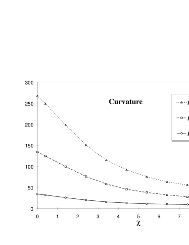
   Figure 1: The curvature for several paths

3. The heat capacity respect to curvature, defined as

   $$C_{\chi}=\frac{-\chi^{2}}{N}\frac{\partial^{2}\ln Z}{\partial\chi^{2}},$$ (4)

   which is shown in fig. 2.

   

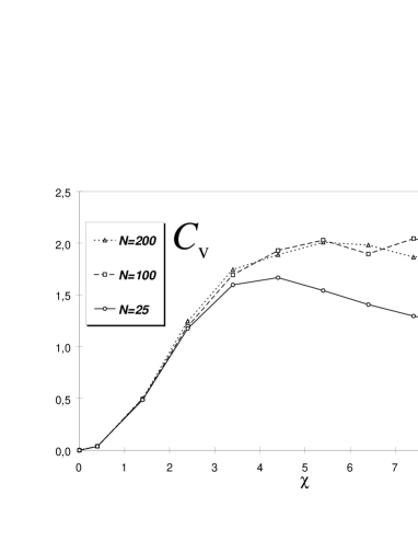
   Figure 2: The specific heat for several paths

4. The gyration radius, shown in figure 3:

   $$<X^{2}>_{c}=\frac{1}{d}\left(<X^{2}>-<X>^{2}\right).$$ (5)

   

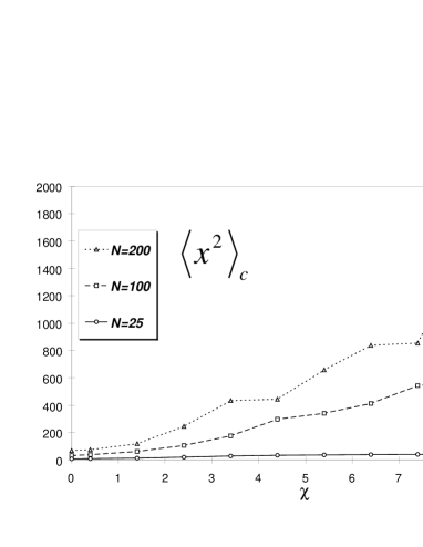
   Figure 3: The gyration radius for several paths

5. Finally, the Hausdorff dimension of the path defined as (see fig. 4):

   $$d_{H}=\lim_{N\rightarrow\infty}2\frac{\ln<X^{2}>_{c}}{\ln N}.$$ (6)

   

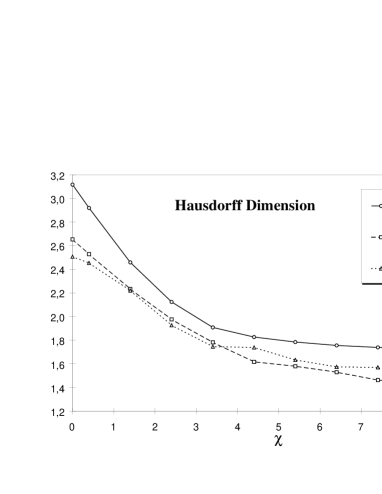
   Figure 4: The Hausdorff dimension for several paths

5 Numerical results and conclusions

There appear two different regimes:

• For small curvature coupling, $d_{H}=2$, i.e. Brownian paths.

• For large curvature coupling, $d_{H}=1$, i.e. Rigid paths.

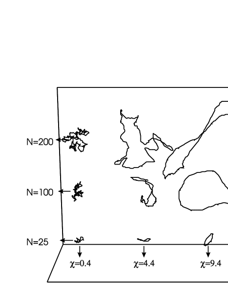
Figure 5: Snapshots for several paths. Notice how the “size” of the paths (the gyration radius) grows with $N$ and how the curvature decreases as $\chi$ grows.

The simple snapshots of the paths (fig. 5) visualize this change of behavior. Furthermore, the specific heat graph, the curvature graph and the gyration radius graph shown all three a clear cross-over separating the two phases. The large correlation in the simulation difficult a finite size analysis of the specific heat the cross-over to exclude the presence of a second order or a continuous phase transition. Nevertheless, it is remarkable the similarity between the specific heat graphs of this model and those of crystaline random surfaces, where a true second order phase transition has been observed.

All our results are compatible with the existence of a critical point at infinite curvature coupling, as it is expected from mean field analysis.

The collaboration of A. Jaramillo in the initial stages of this work is acknowledged. Numerical computations have been performed in the cluster of IBM/RISC 6000 workstations of IFAE and in the CRAY of CESCA. This work has been partially supported by research project CICYT AEN95/0882

References

- [1] A.M. Polyakov, Phys. Lett. 103B (1981) 207.
- [2] A. Billoire, D.J. Gross and E. Marinari, Phys. Lett. 139B (1984) 75.
-
[3]
L. Peliti and S. Leibler, Phys. Rev. Lett. 54
(1985) 1690.
A.M. Polyakov, Nucl. Phys. B268 (1986) 406. - [4] M. Baig, D. Espriu and A. Travesset, Nucl. Phys. B426 (1994) 575.
- [5] R. D. Pisarski, Phys. Rev. D34 (1986) 670.
- [6] F. Alonso and D. Espriu, Nucl. Phys. B283 (1987) 393.
-
[7]
M. Warner, J. Gunn and A. Baumgartner, J. Phys. A:
Math. Gen. 18 (1985) 3007.
J.J. Hermanns and R. Ullman, Physica 18 (1952) 951 -
[8]
J. Ambjørn, B. Durhuus and T. Jonsson, Europhys.
Lett. 3 (1987) 1059.
J. Ambjørn, B. Durhuus and T. Jonsson, J. Phys. A: Math. Gen. 21 (1988) 981. - [9] J. Ambjørn, B. Durhuus and T. Jonsson, Nucl. Phys. B330 (1990) 509.
- [10] M. Baig, J. Clua and A. Jaramillo. “Numerical simulation of random paths with a curvature dependent action”. Preprint UAB-FT 395, submitted to Phys. Lett. B.