Numerical simulation of random paths
with a curvature dependent action

Abstract

We study an ensemble of closed random paths, embedded in $\mbox{\QRC R}^{3}$, with a curvature dependent action. Previous analytical results indicate that there is no crumpling transition for any finite value of the curvature coupling. Nevertheless, in a high statistics numerical simulation, we observe two different regimes for the specific heat separated by a rather smooth structure. The analysis of this fact warns us about the difficulties in the interpretation of numerical results obtained in cases where theoretical results are absent and a high statistics simulation is unreachable. This may be the case of random surfaces.

1 Introduction

It is well known that the addition of an extrinsic curvature term to the Nambu-Goto action (i.e. the area action) for the case of random surfaces controls the formation of spikes, i.e. deformations that are exact zero-modes of the area action and causes the degeneration of the random surface into branched polymers  [1, 2, 3].

The presence of a second order phase transition for a finite value of the curvature-coupling separating a crumpled and a flat phase for the case of fixed connectivity random surfaces in three dimensions has been firmly established by recent large scale numerical simulations  [4, 5].

Nevertheless, the situation is far from being so clear for the case of dynamically triangulated random surfaces with extrinsic curvature (DTRS). Results from numerical simulations of this model are unclear and even the real existence of a phase transition separating the two regimes has been questioned  [6, 7].

It has been pointed out also that these approaches, initially developed to give a lattice discretization for the string theories [8], may have a realization in condensed matter physics as models of membranes or interfaces. In this sense, fixed connectivity random surfaces are called crystalline surfaces and dynamically triangulated surfaces are called fluid surfaces. The comparison between the behavior of DTRS and the true fluid membranes states an interesting question. In fact, the Monte Carlo analysis of the scaling properties of self-avoiding fluid membranes with an extrinsic bending rigidity indicates that fluid membranes are always crumpled at sufficiently long length scales [9, 10]. The observed peak in the specific heat is interpreted as the effect originated when the persistence length describing the exponential decay of the normal-normal two point function in the crumpled regime simply reaches the finite size of the system at the apparent transition. Can this behavior be translated to the case of DTRS?

In this letter we propose a simple scenario: the numerical simulation of the behavior of a set of random paths with an extrinsic curvature term in the action. This system is is particularly adequate to test the numerical techniques used in random surfaces for several reasons:

1. Its numerical simplicity (not triviality!) that allows to perform simulations with several millions of sweeps (simply impossible to do in random surfaces).

2. It is the most natural place to start with random surfaces simulations, as it has been pointed out by several authors [11, 12, 13].

3. It exist a solid framework given by the analytical results obtained by Ambjørn et al. [14].

2 Random Paths with Curvature

The analysis of a random path consisting on straight segments embedded in $\mbox{\QRC R}^{3}$ was performed as a one-dimensional analogue to check the numerical techniques applied in the numerical simulations of triangulated random surfaces [11]. Pisarski [12] proposed the addition of an extra term –proportional to the curvature– to the theory of random paths, claiming that this theory might be relevant to polymer physics. He noticed the observation of asymptotic freedom and pointed out the similarities between this theory and a nonlinear $\sigma$-model with long-range interactions. Furthermore, Alonso and Espriu [13] included random paths as a simple version of the random surface theory in a mean field analysis. They concluded that the Hausdorff dimension of the paths will change from $d_{H}=2$ (Brownian paths) to $d_{H}=1$ at infinite curvature coupling. In 1987 Ambjørn, Durhuus and Jóhnsson [14] performed a complete analytical analysis of this model and they concluded that for finite values of the coupling constant of the curvature term, the theory belongs to the same universality class of simple random walks. A non-trivial scaling limit is only possible if the curvature coupling tends to infinity. They computed exactly the two-point function in this limit. They observed that all the paths have anomalous dimension $\eta=1$, which is consistent with the mean field analysis.

In this letter we perform an actual simulation of a micro-canonical set of random paths with a curvature dependent action. Such an analysis, dealing with finite paths made of a given number of straight segments, allows for a graphical visualization of the role of the curvature term of the action. Geometrical magnitudes such as the curvature or the gyration radius can be directly measured and the scaling behavior explicitly deduced. A close correspondence with the conventions and techniques used in the simulations of random surfaces has been imposed: closed paths of a given number of points, fixed topology, a Metropolis algorithm, etc.

3 Lattice action for closed paths

Pisarski [12] considered a one dimensional analogue of the string action defined in  [2] allowing a path integration over paths $X^{\mu}(\psi)$ as

$$S=\beta\int ds+\chi\int k\,\,ds,$$ (1)

where $s$ is the parameter for which $\left(\frac{dX}{ds}\right)^{2}=1$, and $k$ is the curvature given by $k^{2}=\left(\frac{d^{2}X}{ds^{2}}\right)^{2}$ (both $\beta$ and $\chi$ being positive).

Given an arbitrary parameterization

$$S=\chi\int\frac{(\dot{X}^{2}\ddot{X}^{2}-(\dot{X}\ddot{X})^{2})^{\frac{1}{2}}}{\dot{X}^{2}}dt+\beta\int(\dot{X}^{2})^{\frac{1}{2}}dt,$$ (2)

Pisarski showed, using perturbation theory, that at $\chi^{-1}=0$ the theory is asymptotically free. Therefore, the paths will become smoother as we go to shorter distances, but longer distances are outside the validity of perturbation theory.

Ambjørn et al. [14] studied the non-perturbative regime of this theory but considered open endpoints. Using a lattice-like regularization and a generalized central limit theorem, they concluded that there are actually no other phase transitions than the $\chi^{-1}=0$ point (which it is expected from asymptotic freedom). This implies that the correlation length must increase for small $\chi^{-1}$. A similar result was obtained in the approximation of mean-field theory [13].

The actual action we have simulated is a lattice transcription of the action (2) obtained by simply replacing the derivatives of the path $\dot{X^{\mu}_{i}}$ by finite differences $X^{\mu}_{i+1}-X^{\mu}_{i}$ (and doing analogously with second derivatives):

$$S=\beta\sum_{i=1}^{N}|X_{i}-X_{i-1}|+2\chi\sum_{i=1}^{N}\left|\sin\frac{\theta_{i}}{2}\right|.$$ (3)

where $\theta_{i}$ is the angle between two adjacent segments.

The partition function of this theory is, then, defined as

$$Z=\int\prod^{N-1}_{i=1}d^{3}X_{i}\;e^{-S}.$$ (4)

It is easy to check that, like in the surface case, this action is invariant under reparameterizations which may be thought as a kind of gauge symmetry. This fact allows to fix the coupling $\beta=1$ obtaining, actually, a single parameter action.

We have restricted ourselves to the case of closed paths, i.e. we have require that the neighbor of the $i=N$ point is $i=1$. We have also fixed this point to avoid translational invariance. All these prescriptions are in perfect agreement with the simulation of random surfaces.

From a geometrical point of view, the paths we have simulated consist in closed loops of straight segments embedded in $\mbox{\QRC R}^{3}$, being this topology preserved during the simulation.

4 Numerical results

We have performed numerical simulations for paths embedded in ${\QRC R}^{D}$ ($D=3$) with different number of points: $N=25,100,200$ and for different values of the curvature coupling $\chi$ from 0 to 10, keeping always $\beta=1$. The number of sweeps has been of the order of 2-4 millions for each coupling. The numerical computation of the partition function has been done using a simple Metropolis algorithm [11]. We have not applied histogram or re-summation techniques due to the large fluctuations and large correlations experienced by this system. The use of other methods such as Hybrid Monte Carlo algorithms seems not to improve the results [15]. Main results concerning the geometrical and thermodynamical behavior of the paths are as follows:

1. Length. The measure of the mean length of the paths constitutes a good test of the numerical procedure. It is easy to deduce that independently of the curvature $\chi$ value,

   $$\left<L\right>=-\frac{\partial\ln Z}{\partial\beta}=\frac{(N-1)D}{\beta}.$$ (5)

   Results to compare with the analytical prediction are summarized in table 1.

   Table 1: Some lengths compared with the predicted value

   $$\begin{array}[]{|c|c|c|c|}\hline\cr\chi&N=25\ (72)&N=100\ (297)&N=200\ (597)\\ \hline\cr 0.0&71.9\pm 0.1&296.7\pm 0.2&597.3\pm 0.4\\ 1.4&71.7\pm 0.1&296.5\pm 0.2&595.9\pm 0.5\\ 3.4&72.3\pm 0.2&297.5\pm 0.6&600.1\pm 1.0\\ 5.4&71.6\pm 0.2&297.5\pm 0.8&594.8\pm 1.6\\ \hline\cr\end{array}$$

2. Curvature. The mean total curvature of the path is given by

   $$\left<S_{c}\right>=\left<\int k\,ds\right>=-\frac{\partial\ln Z}{\partial\chi}.$$ (6)

   We have summarized in fig. 1 the results concerning the curvature measurements. Notice the decrease of the mean curvature as the coupling $\chi$ grows. The solid curve represents the limit $\chi\rightarrow\infty$ and $N\rightarrow\infty$ when the path becomes a flat circle and the total curvature is just $2\pi$.

   

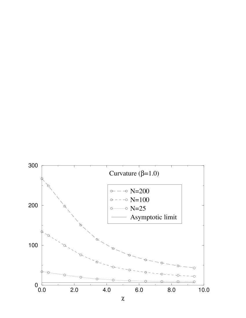
   Figure 1: Curvature for several paths

   

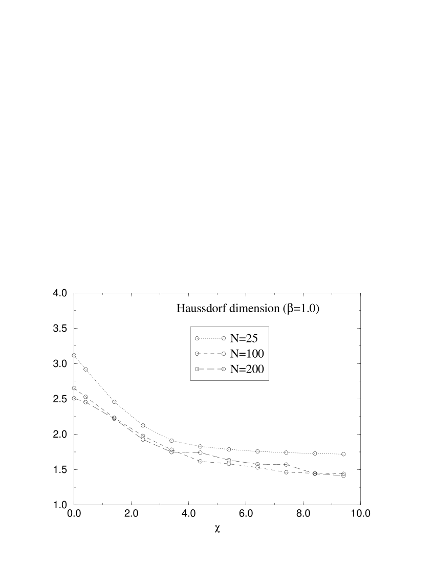
   Figure 2: Hausdorff dimension for several paths

3. Hausdorff Dimension. The square gyration radius is a geometrical magnitude defined as

   $$\left<X^{2}\right>_{c}=\frac{1}{D}\left(\left<X^{2}\right>-\left<\vphantom{X^{2}}X\right>^{2}\right).$$ (7)

   For zero curvature coupling the mean value of the square gyration radius is just [16]

   $$\left<X^{2}\right>_{c}=N\;\frac{(D+1)}{12\beta^{2}},$$ (8)

   in perfect agreement with our results. In the infinite curvature limit  [15]

   $$\left<X^{2}\right>_{c}=(N-1)^{2}\;\frac{D}{(2\pi\beta)^{2}}.$$ (9)

   From the square gyration radius we can extract the Hausdorff dimension (see fig. 2).

   From the analytical results [14] we know that in the continuous limit random paths must be crumpled for all finite curvature couplings (including the case $\chi=0$). This implies $d_{H}=2$ (i.e. the square gyration radius scales as $N$). Rigid paths are expected only at the infinite curvature coupling, and in this case, we expect $d_{H}=1$ (i.e. the square gyration radius scales as $N^{2}$). The analysis of fig. 2 shows an unexpected behavior. For $\chi=0$ the values of the Hausdorff dimension, for the different sizes of the paths, are all higher than $d_{H}=2$. These values decrease when $N$ increases and they are in perfect agreement with eq. (8), so in the infinite volume ($N\to\infty$) the value of the Hausdorff dimension is $d_{H}=2$, as expected for Brownian paths. However, the behavior of paths at non-zero curvature coupling is rather difficult to connect with the above scenario. We observe that for each size $N$, the value of $d_{H}$ decreases as a function of $\chi$ up to an almost constant value for large (but still finite) couplings. For all the sizes studied, these limiting values are lower than $d_{H}=2$ and, for large $N$, they approaches a value close to $d_{H}=1.5$. The effects of dealing with paths of finite size seems to be, then, stronger than naive expectations.

   We have drawn in fig. 3 simple snapshots of the paths for different curvature couplings. They show an apparent change of behavior from crumpled or Brownian paths to rigid paths. For large curvature terms, a closed path build of a finite number of straight segments seems to be frozen.

4. Specific heat. In addition to this geometrical picture, we have measured also the heat capacity with respect to curvature, defined as

   $$C_{\chi}=\frac{-\chi^{2}}{N}\;\;\frac{\partial^{2}}{\partial\chi^{2}}\ln Z,$$ (10)

   where $Z$ is the canonical partition function of the system.

   

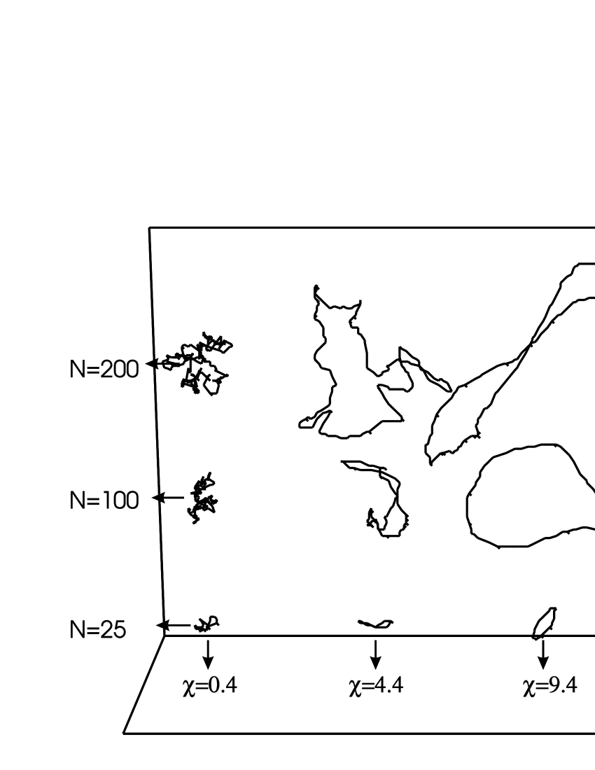
   Figure 3: Simple snapshots for several paths.

   

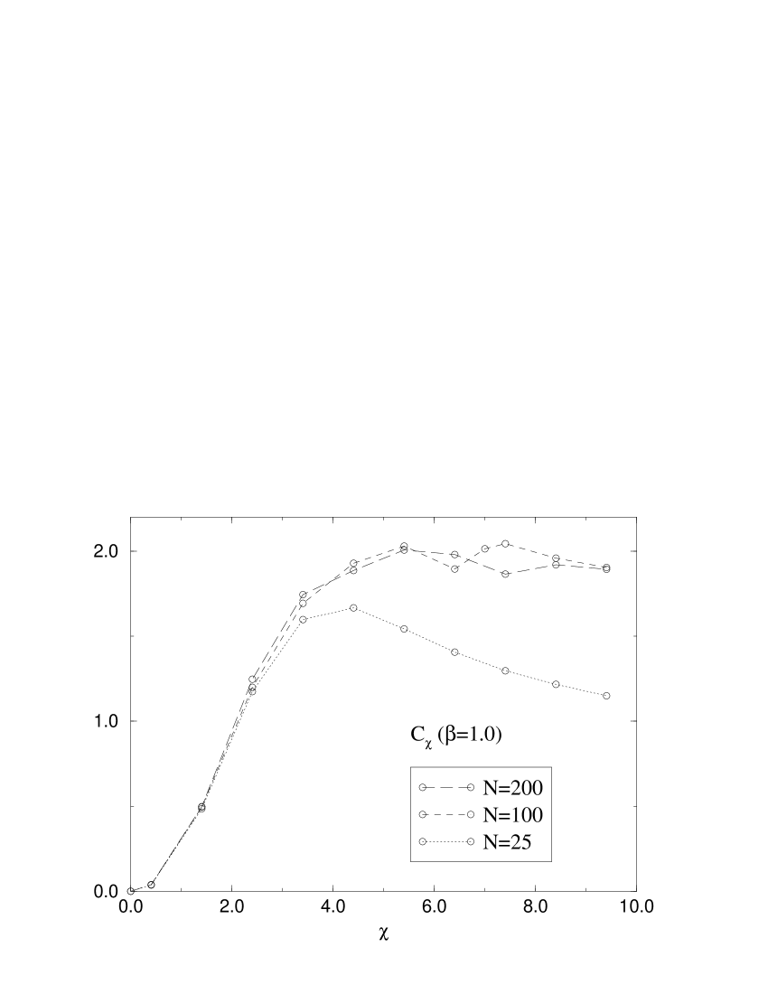
   Figure 4: Specific heat for several paths.

   Its behavior, shown in fig. 4, is really suggestive. Remark, for instance, the saturation for long paths. The shape of this graph is very similar to that corresponding to the self-avoiding fluid membranes [9], for which the authors conclude the absence of a phase transition. Moreover it is also similar to the case of crystalline random surfaces, where there is a true phase transition [17, 4]. This reflects the fact that a crude observation of a structure in the specific heat graph is not relevant enough to characterize a phase transition.

We should remark that a great difficulty in this analysis is the large correlation found in the simulations, specially for large curvature couplings. This is not only due to the poor efficiency of the method, but is mainly due to the finite size effects of the system.

5 Conclusions

We have performed a numerical simulation of an ensemble of closed random paths embedded in $\mbox{\QRC R}^{3}$ weighted with an action proportional to both, the length of the path and the curvature. Several geometrical and thermodynamical magnitudes have been measured: Length, curvature, gyration radius, Hausdorff dimension and specific heat.

This is a privileged framework, because from analytical results we know that there is no true phase transition and that for a finite non-zero curvature coupling these paths will belong to the same universality class than Brownian random walks. In addition, one has the possibility of perform a high statistics simulation. Nevertheless, in an actual numerical simulation, the finite size effects and the large correlations in the system hide the expected behavior.

In addition to the intrinsic interest of such a simulation –that completes previous works on this field [12, 14]– the experience acquired warns us that one must be very careful when dealing with other situations without firmly established analytical results.

Acknowledgments

Two of us (MB, JC) thank J. Ambjørn, D. Espriu, A. Pap and P. Suranyi for useful comments and suggestions. AJ is supported by a doctoral fellowship from IVEI. This work has been partially supported by research project CICYT AEN95/0882.

References

- [1] Peliti L. and Leibler S. Phys. Rev. Lett. 54 1985 1690.
- [2] Polyakov A. M. Nucl. Phys. B268 1986 406.
- [3] David F. Europhys. Lett. 2 1986 577.
- [4] Wheater J. F. Nucl. Phys. B458 1996 671.
-
[5]
Bowick M. J., Catterall S. M.,
Falcioni M., Thorleifsson G. and
Anagnostopoulos K. N. J. Phys. I France 6 1996 1321. -
[6]
Bowick M., Coddington P., Han L., Harris G. and Marinari E.
Nucl. Phys. B394 1993 791. - [7] Anagnostopoulos K., Bowick M., Coddington P., Falcioni M., Han L., Harris G. and Marinari E. Phys. Lett. B317 1993 102.
- [8] Ambjørn J. Quantization of Geometry, Les Houches 1994, hep-th/9411179 preprint.
- [9] Kroll D. M. and Gompper G. Science 255 1992 968.
- [10] Kroll D. M. and Gompper G. Phys. Rev. A46 1992 3119.
- [11] Billoire A., Gross D. J. and Marinari E. Phys. Lett. 139B 1984 75.
- [12] Pisarski R. D. Phys. Rev. D34 1986 670.
- [13] Alonso F. and Espriu D. Nucl. Phys. B283 1987 393.
-
[14]
Ambjørn J., Durhuus B. and Jónsson T.,
Europhys. Lett. 3 1987 1059;
Ambjørn J., Durhuus B. and Jónsson T. J. Phys. A: Math. Gen. 21 1988 981. - [15] Baig and Clua J. in preparation.
- [16] Gross D. J. Phys. Lett. 138B 1984 185.
- [17] Baig M., Espriu D. and Travesset A. Nucl. Phys. B426 1994 575.