Abstract

We present an exact version of the local bosonic algorithm for the simulation of dynamical quarks in lattice QCD. This version is based on a non-hermitian polynomial approximation of the inverse of the quark matrix. A Metropolis test corrects the systematic errors. Two variants of this test are presented. For both of them, a formal proof is given that this Monte Carlo algorithm converges to the right distribution. Simulation data are presented for different lattice parameters. The dynamics of the algorithm and its scaling in lattice volume and quark mass are investigated.

1 Introduction

As the accuracy of quenched QCD simulations improves, the systematic error caused by the quenched approximation becomes more and more important. Accurate full QCD simulations are needed, for which hardware performance improvement appears insufficient. Theoretical and algorithmic progress is necessary.

The search for more efficient full QCD algorithms has motivated substantial activity, both within the classical Hybrid Monte Carlo (HMC) and in the alternative method of the local bosonic algorithm. This last algorithm was proposed by Lüscher in a hermitian version [1]. The idea was to approximate the full QCD partition function using a local bosonic action based on a polynomial approximation of the inverse of the squared Wilson fermion matrix. The aim was to obtain an algorithm which does not need the explicit inversion of the fermion matrix and which only uses local, finite-step-size updates, contrary to HMC. If one evaluates the low-lying spectrum of the matrix, the systematic errors due to the approximation can be corrected, either in the measurement of observables [1] or directly by a Metropolis test [2]. Unfortunately, it turned out that the autocorrelation time was very large [3, 4] and the correction of the systematic errors using the spectrum very costly [5].

Recently, several significant improvements have been proposed to improve the efficiency of this algorithm: (a) an inexpensive stochastic Metropolis test [6]; (b) a non-hermitian polynomial approximation [6]; (c) a simple even-odd preconditioning [7]; (d) a two-step approximation for non-even number of flavors [8]. Preliminary studies combining (a) and (b) looked very promising [9]. Here we combine (a), (b) and (c) for two-flavor QCD, and we present a detailed description of the algorithm and a formal proof of its correctness. We illustrate the effectiveness of our algorithm with representative Monte Carlo results. We successfully model its static properties (the Monte Carlo acceptance), and try to disentangle its dynamics, using both Monte Carlo measurements and a toy-model.

From our analysis it appears that this version of the local bosonic algorithm is a real alternative to the classic HMC. Its scaling in lattice volume and quark mass compares favorably with respect to HMC. Thus our algorithm becomes increasingly attractive at low quark mass on large lattices. In addition, because it uses local updating techniques, it is not affected by the accumulation of roundoff errors which can marr the reversibility of HMC in such cases.

2 Description of the algorithm

2.1 The non-hermitian exact local bosonic algorithm

The full QCD partition function with two fermion flavors is given by

$$Z=\int[dU]|\det D|^{2}e^{-S_{G}[U]}$$ (1)

where $D$ represents the fermion matrix and $S_{G}$ denotes the pure gauge action. This partition function can be approximated introducing a polynomial approximation of the inverse of the fermion matrix.

$$|\det D|^{2}=\det D^{\dagger}\det D\simeq\frac{1}{|\det P(D)|^{2}}$$ (2)

The polynomial $P(z)=\prod_{k=1}^{n}(z-z_{k})$ of degree $n$ is defined in the complex plane and approximates the inverse of $z$. The approximation is controlled by the degree $n$ of the polynomial and the position of its roots in the complex plane. A complete discussion of the choice of the roots is given in [6]. In our work we have chosen the roots on an ellipse centered in $c$ and with focal distance $f$

$$z_{k}=c(1-\cos\theta_{k})-i\sqrt{c^{2}-f^{2}}\sin\theta_{k}$$ (3)

where $\theta_{k}=\frac{2\pi k}{n+1}$. For our simulation at $\beta=0$ we have chosen a circle with $c=1$ and $f=0$. Since we are investigating full QCD with two flavors, the determinant $|\det P(D)|^{2}$ manifestly factorizes into positive pairs, for any choice of the $z_{k}$’s (real or complex) and any degree $n$ (even or odd):

$$|\det P(D)|^{2}=\mbox{constant}\times\prod_{k=1}^{n}\det(D-z_{k})^{\dagger}(D-z_{k})$$ (4)

The $\frac{1}{|\det P(D)|^{2}}$ term of the approximation (2) can be expressed by a Gaussian integral over a set of boson fields $\phi_{k}$ ($k=1,...,n$) with color and Dirac indices and with partition function

$$Z_{b}=\int\prod_{k=1}^{n}[d\phi_{k}][d\phi^{\dagger}_{k}]e^{-\phi^{\dagger}_{k}(D-z_{k})^{\dagger}(D-z_{k})\phi_{k}}$$ (5)

The full QCD partition function (1) is then approximated by

$$Z\simeq\int[dU]Z_{b}[U]e^{-S_{G}[U]}$$ (6)

Making use of the locality of the Lüscher action

$$S_{L}=S_{G}+S_{b}$$ (7)

where

$$S_{b}=\sum_{k=1}^{n}S_{b}^{k}=\sum_{k=1}^{n}\phi^{\dagger}_{k}(D-z_{k})^{\dagger}(D-z_{k})\phi_{k}$$ (8)

we may now simulate the partition function (6) by locally updating the boson fields and the gauge fields, using heat-bath and over-relaxation algorithms.

We consider the update $(U,\phi)\rightarrow(U^{\prime},\phi^{\prime})$ of the gauge and boson fields consisting of a ”trajectory” or sequence of $m$ local updates according to the approximate partition function (6). We choose an update sequence of these fields which satisfies detailed balance with respect to the Lüscher action $S_{L}=S_{G}+S_{b}$. This means that the transition probability from an old configuration $(U,\phi)$ to a new one $(U^{\prime},\phi^{\prime})$ satisfies

$$\frac{P_{(U,\phi)\rightarrow(U^{\prime},\phi^{\prime})}^{L}}{P_{(U^{\prime},\phi^{\prime})\rightarrow(U,\phi)}^{L}}=e^{-(S_{L}(U^{\prime},\phi^{\prime})-S_{L}(U,\phi))}$$ (9)

This is achieved by symmetrically ordering the update steps of the $U$ and $\phi$ fields (over-relaxation and heat-bath for the boson fields; over-relaxation for the gauge fields) so that they be invariant under reversal of the trajectory. Additionally, one can organize the updates on random sublattices. Different organizations are also possible. In our simulations we have tested different combinations of the updating steps. A quite efficient one is composed of one heat-bath of the boson fields, $m$ alternated over-relaxations of the boson and the gauge fields, and a further over-relaxation and heat-bath of the boson fields to symmetrize the trajectory.

The simulation of full QCD can be obtained from (6) by correcting the errors due to the approximation through a Metropolis test at the end of each trajectory. Introducing the error term in the partition function we obtain

$$Z = \int[dU]|\det D|^{2}\frac{|\det P(D)|^{2}}{|\det P(D)|^{2}}e^{-S_{G}[U]}=\int[dU]|\det(DP(D))|^{2}Z_{b}[U]e^{-S_{G}[U]}=$$ (10)

$$= \int[dU][d\phi][d\phi^{\dagger}]|\det(DP(D))|^{2}e^{-S_{L}(U,\phi)}$$

where $\phi$ represents the sets of all boson field families. The correction term $|\det(DP(D))|^{2}$ can be evaluated in two different ways.

The first one consists in estimating the average determinant $<|\det(DP(D))|^{2}>$ using a noisy estimator of the Gaussian integral

$$\int[d\eta][d\eta^{\dagger}]e^{-|[DP(D)]^{-1}\eta|^{2}}$$ (11)

The strategy of this method is to update the $(U,\phi)$ fields such that the probability of finding a particular configuration is proportional to $e^{-S_{L}}$ and then perform a Metropolis test defining an acceptance probability $P^{A}$ in terms of the noisy estimation of the correction $|\det(DP(D))|^{2}$. In this case the full transition probability of the algorithm $P=P^{L}P^{A}P^{HB}$ satisfies detailed balance

$$\frac{<P_{(U,\phi)\rightarrow(U^{\prime},\phi^{\prime})}>}{<P_{(U^{\prime},\phi^{\prime})\rightarrow(U,\phi)}>}=\frac{|\det(D^{\prime}P(D^{\prime}))|^{2}e^{-S_{L}(U^{\prime},\phi^{\prime})}}{|\det(DP(D))|^{2}e^{-S_{L}(U,\phi)}}$$ (12)

after averaging over the $\eta$ fields which are generated by a Gaussian heatbath according to the probability density $P^{HB}$. Here we call $D^{\prime}$ and $D$ the fermion matrix for the new and old gauge configurations respectively.

The second method consists in expressing the correction term $|\det(DP(D))|^{2}$ directly by a Gaussian integral and incorporating the dynamics of the correction field $\eta$ in the partition sum (10)

$$Z = \int[dU][d\eta][d\eta^{\dagger}][d\phi][d\phi^{\dagger}]e^{-S_{L}[U]}e^{-|[DP(D)]^{-1}\eta|^{2}}=$$ (13)

$$= \int[dU][d\eta][d\eta^{\dagger}][d\phi][d\phi^{\dagger}]e^{-S_{exact}(U,\phi,\eta)}$$

by defining a new exact action

$$S_{exact}(U,\phi,\eta)=S_{L}(U,\phi)+S_{C}(U,\eta)$$ (14)

where

$$S_{C}(U,\eta)=|[DP(D)]^{-1}\eta|^{2}$$ (15)

is the correction action. In carrying out the simulation one generates configurations of $(U,\phi)$ and $\eta$ such that the probability of finding a particular configuration is proportional to $\exp(-S_{exact})$. Also in this case the strategy is to alternatively update the $(U,\phi)$ fields and the $\eta$ fields. The Metropolis acceptance probability $P^{A}$ is not defined using a noisy estimation of the correction $|\det(DP(D))|^{2}$, but directly using the exact action (14) so that the transition probability of the algorithm $P=P^{L}P^{A}P^{HB}$ satisfies detailed balance

$$\frac{P_{(U,\phi,\eta)\rightarrow(U^{\prime},\phi^{\prime},\eta^{\prime})}}{P_{(U^{\prime},\phi^{\prime},\eta^{\prime})\rightarrow(U,\phi,\eta)}}=\frac{e^{-S_{exact}(U^{\prime},\phi^{\prime},\eta^{\prime})}}{e^{-S_{exact}(U,\phi,\eta)}}$$ (16)

without the need to average over $\eta$. We have tested both methods and both seem equally efficient.

2.1.1 Noisy Metropolis test

The idea of the noisy estimator is to generate for each trajectory a field $\eta$ using a heatbath according to the Gaussian distribution

$$P_{\eta}^{HB}(U)=\frac{R}{|\det DP(D)|^{2}}e^{-|[DP(D)]^{-1}\eta|^{2}}$$ (17)

(where $R$ is a normalization constant), and accept the new configuration $(U^{\prime},\phi^{\prime})$ with the acceptance probability

$$P^{A}_{(U,\phi)\rightarrow(U^{\prime},\phi^{\prime})} =\min\left(1,e^{-|[D^{\prime}P(D^{\prime})]^{-1}\eta|^{2}+|[DP(D)]^{-1}\eta|^{2}}\right)$$ (18)

$$=\min\left(1,E^{A}_{U\rightarrow U^{\prime}}\right)$$

The probability density responsible for the Metropolis correction is then the product

$$P^{C}_{(U,\phi)\rightarrow(U^{\prime},\phi^{\prime})}=P^{HB}_{\eta}(U)\,P^{A}_{(U,\phi)\rightarrow(U^{\prime},\phi^{\prime})}$$ (19)

For a single trajectory the correction term is estimated by one $\eta$ field only. Because a trajectory making a transition $(U,\phi)\rightarrow(U^{\prime},\phi^{\prime})$ can occur infinitely many times one can average over the $\eta$ field and using

$$<P^{C}_{(U,\phi)\rightarrow(U^{\prime},\phi^{\prime})}>=$$ (20)

$$=\frac{R}{|\det DP(D)|^{2}}\left[\int_{E^{A}>1}[d\eta][d\eta^{\dagger}]e^{-|[DP(D)]^{-1}\eta|^{2}}+\int_{E^{A}<1}[d\eta][d\eta^{\dagger}]e^{-|[D^{\prime}P(D^{\prime})]^{-1}\eta|^{2}}\right]$$

and

$$E^{A}_{U\rightarrow U^{\prime}}=\frac{1}{E^{A}_{U^{\prime}\rightarrow U}}$$ (21)

one can see that detailed balance (12) is satisfied. Because in the probability density (17) we have the inverse of $DP(D)$ we can organize the Gaussian heatbath by generating a Gaussian spinor $\chi$ with variance one and obtaining the $\eta$ field by assigning $\eta=DP(D)\chi$. It is then convenient to express the acceptance probability $P^{A}$ using this substitution

$$P^{A}_{(U,\phi)\rightarrow(U^{\prime},\phi^{\prime})}=\min\left(1,e^{-|W\chi|^{2}+|\chi|^{2}}\right)$$ (22)

where $W=[D^{\prime}P(D^{\prime})]^{-1}DP(D)$ as suggested in [6].

2.1.2 Non-noisy Metropolis test

Let us consider now the updating of the $\eta$ field when its dynamics is incorporated in the partition sum by the exact action (14). We want to update this field by a Gaussian heatbath. The probability density $P^{HB}_{\eta\rightarrow\eta^{\prime}}(U,U^{\prime})$ for obtaining a field $\eta^{\prime}$ at the end of a trajectory, starting from the field $\eta$ at the beginning of a trajectory, can be chosen trivially independent from $\eta$ but has to depend upon the gauge fields $U$ or $U^{\prime}$. In addition it has to satisfy exactly detailed balance with respect to the action $S_{C}$ when keeping the gauge fields $U$ and $U^{\prime}$ fixed. This is achieved by introducing an arbitrary ordering of the gauge configurations, for example

$$U\succ U^{\prime}\mbox{ if }S_{G}(U)>S_{G}(U^{\prime})$$ (23)

and choosing the Gaussian heatbath probability density

$$P_{\eta\rightarrow\eta^{\prime}}^{HB}(U,U^{\prime})=\left\{\begin{array}[]{lr}\frac{R}{|\det DP(D)|^{2}}e^{-S_{C}(U,\eta^{\prime})}&\mbox{ if }U\succeq U^{\prime}\\ \frac{R}{|\det D^{\prime}P(D^{\prime})|^{2}}e^{-S_{C}(U^{\prime},\eta^{\prime})}&\mbox{ if }U\prec U^{\prime}\end{array}\right.$$ (24)

Here $R$ is a normalization constant and $S_{C}$ is defined in (15). Detailed balance is then satisfied for fixed gauge fields

$$\frac{P_{\eta\rightarrow\eta^{\prime}}^{HB}(U,U^{\prime})}{P_{\eta^{\prime}\rightarrow\eta}^{HB}(U^{\prime},U)}=\left\{\begin{array}[]{lr}e^{-(S_{C}(U,\eta^{\prime})-S_{C}(U,\eta))}&\mbox{ if }U\succeq U^{\prime}\\ e^{-(S_{C}(U^{\prime},\eta^{\prime})-S_{C}(U^{\prime},\eta))}&\mbox{ if }U\prec U^{\prime}\end{array}\right.$$ (25)

The crucial point in this method is that the arbitrary ordering of the gauge fields and the choice (24) ensure that in the ratio (25) the unwanted determinants cancel. The cancellation of the determinants allows us to construct a non-noisy algorithm. Because in the action $S_{C}$ we have the inverse of $DP(D)$ (or $D^{\prime}P(D^{\prime})$) the Gaussian heatbath is easily organized as follows: one generates a Gaussian spinor $\chi$ with variance one and obtains the $\eta^{\prime}$ field by assigning

$$\eta^{\prime} = \left\{\begin{array}[]{lr}DP(D)\chi&\mbox{ if }U\succeq U^{\prime}\\ D^{\prime}P(D^{\prime})\chi&\mbox{ if }U\prec U^{\prime}\end{array}\right.$$ (28)

For each trajectory a Gaussian spinor $\chi$ is chosen. At the end of each trajectory a Metropolis test is performed to be able to correct the approximate update of the $U$ and $\phi$ fields. In order to ensure that detailed balance is satisfied with respect to the exact action $S_{exact}$ we accept the proposed change in the $U$ and $\phi$ fields with an acceptance probability $P^{A}_{(U,\phi,\eta)\rightarrow(U^{\prime},\phi^{\prime},\eta^{\prime})}$ which is chosen such that

$$\left.\frac{P_{(U,\phi)\rightarrow(U^{\prime},\phi^{\prime})}^{L}P_{\eta\rightarrow\eta^{\prime}}^{HB}(U,U^{\prime})P^{A}_{(U,\phi,\eta)\rightarrow(U^{\prime},\phi^{\prime},\eta^{\prime})}}{P_{(U^{\prime},\phi^{\prime})\rightarrow(U,\phi)}^{L}P_{\eta^{\prime}\rightarrow\eta}^{HB}(U^{\prime},U)P^{A}_{(U^{\prime},\phi^{\prime},\eta^{\prime})\rightarrow(U,\phi,\eta)}}\right|_{\chi}=e^{-(S_{exact}(U^{\prime},\phi^{\prime},\eta^{\prime})-S_{exact}(U,\phi,\eta))}$$ (29)

For every choice of Gaussian spinor $\chi$. We can choose the probability $P^{A}$ dependent on $\eta$ and $\eta^{\prime}$ according to

$$P^{A}_{(U,\phi,\eta)\rightarrow(U^{\prime},\phi^{\prime},\eta^{\prime})}=\left\{\begin{array}[]{lr}\min\left(1,e^{-S_{C}(U^{\prime},\eta^{\prime})+S_{C}(U,\eta^{\prime})}\right)&\mbox{ if }U\succeq U^{\prime}\\ \min\left(1,e^{-S_{C}(U^{\prime},\eta)+S_{C}(U,\eta)}\right)&\mbox{ if }U\prec U^{\prime}\end{array}\right.$$ (30)

For every choice of Gaussian spinor $\chi$ it is clear that the probability $P^{A}$ (30) satisfies

$$\frac{P^{A}_{(U,\phi,\eta)\rightarrow(U^{\prime},\phi^{\prime},\eta^{\prime})}}{P^{A}_{(U^{\prime},\phi^{\prime},\eta^{\prime})\rightarrow(U,\phi,\eta)}}=\left\{\begin{array}[]{lr}e^{-(S_{C}(U^{\prime},\eta^{\prime})-S_{C}(U,\eta^{\prime}))}&\mbox{ if }U\succeq U^{\prime}\\ e^{-(S_{C}(U^{\prime},\eta)-S_{C}(U,\eta))}&\mbox{ if }U\prec U^{\prime}\end{array}\right.$$ (31)

and using eq. (9) and (25) we prove that detailed balance (29) holds.

It is convenient to express the acceptance probability (30) using (28)

$$P^{A}_{(U,\phi,\eta)\rightarrow(U^{\prime},\phi^{\prime},\eta^{\prime})}=\left\{\begin{array}[]{lr}\min\left(1,e^{-|W\chi|^{2}+|\chi|^{2}}\right)&\mbox{ if }U\succeq U^{\prime}\\ \min\left(1,e^{+|W^{-1}\chi|^{2}-|\chi|^{2}}\right)&\mbox{ if }U\prec U^{\prime}\end{array}\right.$$ (32)

where $W=[D^{\prime}P(D^{\prime})]^{-1}DP(D)$ as suggested in [9].

2.1.3 Summary

The algorithm can be summarized as follows:

• Generate a new Gaussian spinor $\chi$ with variance one.

• Update locally the boson and gauge fields $m$ times in a reversible way.

• Accept/reject the new configuration according to the Metropolis acceptance probability (22) for the noisy version or (32) for the non-noisy version.

In order to evaluate the Metropolis acceptance probability we have to solve linear system involving $DP(D)$ or $D^{\prime}P(D^{\prime})$, for which we use the BiCGstab algorithm [10]. This linear system is very well conditioned because $P(D^{\prime})$ (or $P(D)$) approximates the inverse of $D^{\prime}$ (or $D$). The cost for solving it is moderate and scales like the local updating algorithms in the volume and quark mass.

We emphasize that the algorithm remains exact for any choice of the polynomial $P$. The only requirement is that its roots $z_{k}$ come in complex conjugate pairs or be real [Note that for $n_{f}$ even, real roots and an odd degree $n$ are possible]. If the polynomial approximates the inverse of the fermion matrix well, the acceptance of the Metropolis correction will be high; if not the acceptance will be low. The number and location of the roots $z_{k}$ in the complex plane determine the quality of the approximation and hence the acceptance. Since the algorithm is exact for all polynomial, we do not need any a priory knowledge about the spectrum of the fermion matrix.

2.2 Local updating algorithms

We discuss in this section how we have organized the local updating algorithm for the boson and gauge fields. For the updating of these fields we use standard heatbath and over-relaxation algorithms.

2.2.1 Boson field update

We have a set of $n$ families of boson fields $\phi=\{\phi_{k}\}$, each one associated with a root of the polynomial. Different families do not interact with each other. For a given family $k$, the boson field $\phi_{k}$ couples only to the gauge fields. The bosonic action $S_{b}^{k}$ has a next-to-nearest neighbor interaction term which couples a field $\phi_{k}(x)$ at point $x$ with all its neighbors $\phi_{k}(y)$ at points $y$ within distance $|x-y|\leq\sqrt{2}$ (Euclidean-norm). The local updating algorithm can then be organized by visiting simultaneously all lattice points at a mutual distance larger than $\sqrt{2}$. Dividing the lattice in $2^{4}$-hypercubes and labeling their $8$ diagonals, all points sitting on the diagonals with the same label have the wanted mutual distance. This organization is particularly convenient for a MIMD parallel machine, since it requires few synchronizations. For SIMD machines much simpler organizations are possible. The set of all these diagonals defines $8$ sublattices. These sublattices are visited randomly to ensure reversibility. As a function of $\phi_{k}(x)$ when all the fields on different sublattices are kept fixed, the local boson action takes the form

$$S_{b}^{k}=A_{k}|\phi_{k}(x)|^{2}+[b_{k}]^{\dagger}\phi_{k}(x)+[\phi_{k}(x)]^{\dagger}b_{k}+\mbox{constant}$$ (33)

Using the notation of the Wilson fermion matrix $D$ acting on a field $\phi$ at a point $x$

$$[D\phi](x)=\phi(x)-K\sum_{\mu=0}^{3}[U(x,\mu)(1-\gamma_{\mu})\phi(x+\hat{\mu})+U(x-\hat{\mu},\mu)^{\dagger}(1+\gamma_{\mu})\phi(x-\hat{\mu})]$$ (34)

we have after some simple algebra

$$A_{k}=1+16K^{2}-2Re(z_{k})+|z_{k}|^{2}$$

and

$$b_{k}=[D^{\dagger}D\phi_{k}](x)-\bar{z}_{k}[D\phi_{k}](x)-z_{k}[D^{\dagger}\phi_{k}](x)-(1+16K^{2}-2Re(z_{k}))\phi_{k}(x)$$

The heatbath is then simply given by

$$\phi_{k}(x)\longleftarrow A_{k}^{-1/2}\chi-A_{k}^{-1}b_{k}$$ (35)

where $\chi$ is a Gaussian spinor with variance one. The over-relaxation is given by

$$\phi_{k}(x)\longleftarrow-\phi_{k}(x)-2A_{k}^{-1}b_{k}$$ (36)

2.2.2 Gauge field update

The updating of the gauge fields can be organized by dividing the lattice into even and odd sites. This defines two sublattices. All gauge links $U(x,\mu)$ starting from a sublattice can be updated simultaneously for a fixed direction $\mu$. When all other links are kept fixed the action takes the form

$$S=Re\left(tr\{U(x,\mu)(F_{U}+F_{\phi})^{\dagger}\}\right)+\mbox{constant}$$ (37)

where $F_{U}$ is the usual gauge link staple around $U(x,\mu)$ and $F_{\phi}$ is the staple given by the boson fields, which can be expressed by the matrix $F_{\phi}=\sum_{k}v_{k}[w_{k}]^{\dagger}$ with

$$v_{k} = \left\{(1-\frac{K}{2})-z_{k}-[(1+\frac{K}{2})-z_{k}]\gamma_{\mu}\right\}\phi_{k}(x)-K(1-\gamma_{\mu})B^{k}_{\mu}(x)$$

$$w_{k} = \left\{(1-\frac{K}{2})-z_{k}+[(1+\frac{K}{2})-z_{k}]\gamma_{\mu}\right\}\phi_{k}(y)-K(1+\gamma_{\mu})B^{k}_{\mu}(y)$$

where $y=x+\hat{\mu}$ and

$$B^{k}_{\mu}(z)=\sum_{\nu\neq\mu}\{U(z,\nu)(1-\gamma_{\nu})\phi_{k}(z+\hat{\nu})+U(z-\hat{\nu},\nu)^{\dagger}(1+\gamma_{\nu})\phi_{k}(z-\hat{\nu})\}$$

Once the staple $F_{U}+F_{\phi}$ is evaluated the link $U(x,\mu)$ can be updated using SU(2) subgroups over-relaxation [11].

2.3 Even-odd preconditioning

As we will see in Section 5.4, the computational effort for obtaining decorrelated gauge configurations is proportional to $n^{2}$ (for fixed quark mass), where $n$ is the number of bosonic fields. The number of bosonic fields needed in the approximation depends on the condition number of the fermion matrix. A way to lower the number of fields is to perform a preconditioning of the fermion matrix. To preserve the locality of the updating algorithm it is necessary that the preconditioned matrix remain local. A well-known possibility is even-odd preconditioning . The lattice is labeled by even and odd points and a field $\phi$ can be written in a even-odd basis as

$$\phi=\left(\begin{array}[]{c}\phi_{e}\\ \phi_{o}\end{array}\right)$$ (38)

where $\phi_{e}$ ($\phi_{o}$) denotes the part of the field $\phi$ living on the even (odd) sublattice, respectively. In the even-odd basis the fermion matrix $D$ can be written as

$$D=\left(\begin{array}[]{cc}1&-KM_{eo}\\ -KM_{oe}&1\end{array}\right)$$ (39)

where $M_{eo}$ and $M_{oe}$ are the off-diagonal part of the fermion matrix (34) connecting odd to even sites or even to odd sites, respectively. Using the identity

$$\det\left(\begin{array}[]{cc}X&Y\\ W&Z\end{array}\right)=\det X\det\left(Z-WX^{-1}Y\right)$$ (40)

(where $X,Y,W$ and $Z$ are matrices) we obtain

$$\det D=\det\left(1-K^{2}M_{oe}M_{eo}\right)=:\det\hat{D}$$ (41)

The preconditioned matrix $\hat{D}$ is local and lives only on half of the lattice and involves next-to-nearest neighbor interactions. To simulate full QCD we could introduce a local bosonic action using the preconditioned fermion matrix $\hat{D}$.

$$\hat{S}_{b}=\sum_{k=1}^{n}\phi_{k}^{\dagger}(\hat{D}-z_{k})^{\dagger}(\hat{D}-z_{k})\phi_{k}$$ (42)

but unfortunately the $\hat{D}^{\dagger}\hat{D}$ term connects $(\mbox{next})^{3}$-to-nearest neighbor sites, which makes the local updating too complex. A very simple way to save the situation is to use eq. (40) again and observe that

$$\det(\hat{D}-z_{k})=\det\left((1-z_{k})-K^{2}M_{oe}M_{eo}\right)=$$

$$=\det\left(\begin{array}[]{cc}1-r_{k}&-KM_{eo}\\ -KM_{oe}&1-r_{k}\end{array}\right)=\det(D-r_{k})$$ (45)

where the root $r_{k}$ is chosen such that

$$(1-r_{k})^{2}=1-z_{k}$$ (46)

The last term of (45) allows us to define the local bosonic action for the preconditioned case without using explicitly the matrix $\hat{D}$ but simply redefining the roots of the polynomial from $z_{k}$ to $r_{k}$ of the non-preconditioned local action (8).

$$\hat{S}_{b}=\sum_{k=1}^{n}\phi_{k}^{\dagger}(D-r_{k})^{\dagger}(D-r_{k})\phi_{k}$$ (47)

This simple trick is only possible in the non-hermitian version of the algorithm. In the hermitian version a more complicated method has to be used [7].

The Metropolis test of the preconditioned case must be performed using the $\hat{D}$ matrix. One uses in the test the acceptance (22) or (32) with the preconditioned matrix

$$W=[\hat{D}^{\prime}P(\hat{D}^{\prime})]^{-1}\hat{D}P(\hat{D})$$ (48)

where $P(\hat{D})$ is the polynomial with the original $z_{k}$ roots.

3 Results for the exact local bosonic algorithm.

Numerical simulations using the exact local bosonic algorithm in the non-noisy version described in the previous section have been performed on $4^{4}$, $4^{3}\times 16$ and $8^{4}$ lattices for different $\beta$ and $k$ values. For the $4^{4}$ and $4^{3}\times 16$ lattices we concentrated on $\beta=0$ and $\beta=5$ and for the $8^{4}$ only on $\beta=0$ and $\beta=5.3$. We have performed the majority of the simulations reported upon here at $\beta=0$ for the following reasons:
i) at $\beta=0$ we know the critical hopping parameter $K_{c}$ ($K_{c}=1/4$), and the form of the spectrum of the fermion matrix (it is contained in a circle centered at $(1,0)$ of radius $4K$, and appears to be distributed uniformly within that circle). So the optimal location of the polynomial roots $z_{k}$ is easy in that case: we choose them on the circle $c=1,f=0$ in eq.(3)
ii) at $\beta=0$ there is no danger of running into the deconfined phase before reaching $K=K_{c}$. This makes the comparison among several volumes simpler.
iii) $\beta=0$ represents the hardest case for the inversion of the fermion matrix, and is thus a good test of our algorithm.

We explored the acceptance of the Metropolis correction test and the number of iteration of the BiCGStab algorithm used in the test for inverting $DP(D)$. The study was performed by varying the degree $n$ of the polynomial and the hopping parameter $k$. The results are shown in Table 1 to Table 3. The trajectory length of all the runs is chosen to be 10. The stopping norm of the residual of the BiCGStab is chosen to be $10^{-18}$.

In Tables 1 and 2 we present the results obtained from simulations without using even-odd preconditioning, on $4^{4}$ and $8^{4}$ lattices respectively. One observes that the acceptance increases quite rapidly with the degree of the polynomial, above some threshold. On the other hand, the number of iterations needed to invert $DP(D)$ remains very low for high enough acceptance. These data show clearly that the overhead due to the Metropolis test remains negligible provided that the degree of the polynomial is tuned to have sufficient acceptance.

In Table 3 we present the results obtained from simulations using even-odd preconditioning. For comparison, the parameters of the simulations were chosen equal to some simulation parameters presented in Table 1. The effect of the preconditioning is to improve the approximation so that fewer fields are needed for the same acceptance. From the data we see that the preconditioning reduces the number of fields by at least a factor two.

Comparative examples of the plaquette values obtained using the exact local bosonic algorithm and the HMC algorithm are given in Table 4. For any choice of polynomial the plaquette remains consistent with the HMC data. However, the autocorrelation increases rapidly when the acceptance of the Metropolis test decreases. To optimize the efficiency of the algorithm one has to tune the degree of the polynomial to obtain a certain acceptance. The choice of the optimal acceptance is discussed in detail in the next section.

In Fig. 1 we show the gain in work due to the preconditioning as a function of the inverse quark mass (in the range of $\kappa$ values explored, $m_{q}$ is nearly proportional to $(1-K/K_{c})$). The simulation is done at $\beta=0$ on a lattice $4^{3}\times 16$ with the optimal polynomial. The work is in units of fermion matrix multiplications. Simulations with HMC were performed at the same parameters to compare the two algorithms. It turned out that the exact preconditioned local bosonic algorithm is as efficient as the HMC. Of cource, a more comprehensive comparison is needed.

In Table 5 we present a comparative example between the non-hermitian and the hermitian version of the local bosonic action, without preconditioning. The simulations are done on a $4^{4}$ lattice at $\beta=5$ and $K=0.15$. The superiority of the non-hermitian exact version is evident.

lattice	$\beta$	$K$	$n$	acceptance	$I_{BiCGStab}$
$4^{4}$	0	0.215
			20	0.04(3)	53.0(9)
			24	0.20(5)	3.00(1)
			28	0.43(7)	2.00(1)
			36	0.92(4)	1.00(1)
			40	0.96(3)	1.00(1)
			44	0.94(4)	1.00(1)
			48	0.98(2)	1.00(1)
$4^{4}$	0	0.230
			44	0.20(6)	3.00(1)
			46	0.31(7)	2.42(2)
			48	0.40(7)	2.20(3)
			50	0.60(9)	1.71(1)
			52	0.65(7)	1.54(3)
			54	0.67(10)	1.42(2)
			56	0.73(4)	1.09(1)
			60	0.78(6)	1.00(1)
			70	0.90(4)	1.00(1)
$4^{4}$	5	0.150
			8	0.03(1)	65(8)
			10	0.22(2)	3.03(2)
			12	0.46(3)	2.00(1)
			16	0.81(2)	1.00(1)
			20	0.93(1)	1.00(1)
$4^{4}$	5	0.160
			12	0.09(2)	43(5)
			14	0.20(2)	3.10(4)
			16	0.45(3)	2.00(1)
			20	0.75(2)	1.00(1)
			24	0.86(2)	1.00(1)

Table 1: Acceptance and number of iterations of the BiCGStab algorithm $I_{BiCGStab}$. $4^{4}$ lattice simulation without even-odd preconditioning.

lattice	$\beta$	$K$	$n$	acceptance	$I_{BiCGStab}$
$8^{4}$	0	0.215
			28	0.00(1)	75(1)
			32	0.15(8)	3.52(10)
			36	0.45(1)	2.00(2)
			40	0.65(8)	1.25(3)
			44	0.85(8)	1.00(1)
			48	0.93(4)	1.00(1)
			52	0.98(2)	1.00(1)
			56	0.97(3)	1.00(1)
$8^{4}$	5.3	0.156
			28	0.42(1)	2.00(1)
			34	0.74(1)	1.00(1)
			40	0.87(1)	1.00(1)
$8^{4}$	5.3	0.158
			24	0.04(1)	8.01(1)
			32	0.43(1)	1.97(3)
			38	0.71(1)	1.00(1)
			44	0.86(1)	1.00(1)

Table 2: Acceptance and number of iterations of the BiCGStab algorithm $I_{BiCGStab}$. $8^{4}$ lattice simulation without even-odd preconditioning.

lattice	$\beta$	$K$	$n$	acceptance	$I_{BiCGStab}$
$4^{4}$	0	0.215
			6	0.00(1)	88(1)
			10	0.41(2)	3.24(2)
			14	0.74(1)	2.00(1)
			20	0.96(1)	1.00(1)
$4^{4}$	0	0.230
			18	0.22(2)	4.75(3)
			24	0.60(1)	2.48(4)
			30	0.75(1)	1.87(2)
			36	0.88(1)	1.00(1)

Table 3: Acceptance and number of iterations of the BiCGStab algorithm $I_{BiCGStab}$. $4^{4}$ lattice simulation with even-odd preconditioning.

lattice	$\beta$	$K$	$n$	plaq	$\tau_{int}$
$4^{4}$	5	0.15
			8	0.413(10)	58(5)
			10	0.416(2)	6(1)
			12	0.416(2)	5(1)
			16	0.415(2)	3(1)
			20	0.416(2)	3(1)
			HMC	0.4155(8)	7(1)
$8^{4}$	5.3	0.158
			24	0.4933(?)	$>$300
			32	0.4918(9)	40(5)
			38	0.4909(4)	18(2)
			44	0.4906(4)	16(2)
			HMC	0.4909(2)	?

Table 4: Comparative examples between the plaquette values obtained using our exact local bosonic algorithm and the HMC algorithm. The integrated autocorrelation time is given in units of trajectories. Question marks denote informations which are not available or can not be determined. The acceptance of the Metropolis test for these simulations is given in Tables 1 and 2. The HMC data on the $8^{4}$ lattice is taken from [12].

algorithm	polynom	plaquette	acceptance
non-hermitian	$n=8$	0.413(10)	0.03(1)
exact	$n=10$	0.416(2)	0.22(2)
version	$n=12$	0.416(2)	0.46(3)
	$n=16$	0.415(2)	0.81(2)
	$n=20$	0.416(2)	0.93(1)
hermitian	$n=6,\epsilon=0.05$	0.4239(5)	-
version	$n=14,\epsilon=0.05$	0.4180(7)	-
	$n=50,\epsilon=0.05$	0.4162(12)	-
	$n=80,\epsilon=0.05$	0.4163(10)	-
	$n=50,\epsilon=0.005$	0.413(1)	-
	$n=80,\epsilon=0.005$	0.413(2)	-
	$n=50,\epsilon=0.01$	0.415(1)	-
	$n=80,\epsilon=0.01$	0.415(1)	-
HMC		0.4155(8)

Table 5: Comparative example between the non-hermitian exact local bosonic algorithm, the hermitian local bosonic algorithm and the HMC. Simulation on a $4^{4}$ lattice at $\beta=5$ and $K=0.15$. The autocorrelation time of the data in the hermitian case could not always be determined. For $n\geq 50$ it is of the order of some hunderts of sweeps. The autocorrelation of the data in the non-hermitian case is reported in the Table above.

4 Predicting the Metropolis acceptance

Let us write generically the Metropolis acceptance probability (eq. (22) or (32)) as $P_{acc}=\min(1,e^{-\Delta E})$, with $\Delta E=\chi^{\dagger}(W^{\dagger}W-1)\chi$. Detailed balance requires $<e^{-\Delta E}>=1$, so that $<(\Delta E)^{2}>\simeq 2<\Delta E>$. Then, assuming the distribution of $\Delta E$ to be Gaussian, which is certainly reasonable for systems large compared to the correlation length $\sim m_{q}^{-1}$, one can easily derive (see Appendix A)

$$<P_{acc}>\simeq erfc\left(\sqrt{\frac{<(\Delta E)^{2}>}{8}}\right)$$ (49)

We can estimate $<(\Delta E)^{2}>$ here, because the Chebyshev-like approximation we use for $D^{-1}$ has a known error bound. Recall ([6], eq.(29)) that for any eigenvalue $\lambda$ of $D$, one has

$$\alpha\equiv|\lambda P(\lambda)-1|\leq\tilde{\alpha}\equiv 2~{}\left(\frac{a+\sqrt{a^{2}-c^{2}}}{d+\sqrt{d^{2}-c^{2}}}\right)^{n+1}$$ (50)

where the spectrum of $D$ is contained in an ellipse ${\partial\cal S}$ of center $(d,0)$, large semi-axis $a<d$, and focal distance $c\leq a$. For simplicity we consider here the strong coupling case $\beta=0$. Then the spectrum of $D$ is contained in a circle ($c=0$), and $\frac{a}{d}=\frac{K}{K_{c}}$, with $K_{c}(\beta=0)=1/4$. One can then expect, for the eigenvalues $\tilde{\lambda}$ of $(W^{\dagger}W-1)$ which contains 4 factors of the form $DP(D)$:

$$|\tilde{\lambda}|\leq 4\tilde{\alpha}$$ (51)

Then, assuming that the eigenvalues $\tilde{\lambda}$ fluctuate independently of each other, it follows $<(\Delta E)^{2}>\leq 192V\tilde{\alpha}^{2}$, where $V$ is the number of lattice sites, or at $\beta=0$:

$$<(\Delta E)^{2}>\leq 768V\left(\frac{K}{K_{c}}\right)^{2n+2}$$ (52)

In fact, the bound (50) becomes much tighter for interior eigenvalues of $D$, far from the boundary ${\partial\cal S}$. To model this effect, we introduce a “fudge factor” $f\leq{\cal O}(1)$ in $\tilde{\alpha}$. It will also account for possible correlations between $D$ and $D^{\prime}$ at the beginning and end of a trajectory (ie. between successive Metropolis tests). Substituting in (49) we finally obtain

$$<P_{acc}>\simeq erfc\left(f\sqrt{96V}\left(\frac{K}{K_{c}}\right)^{n+1}\right)$$ (53)

It becomes clear then that the acceptance will change very abruptly with the number $n$ of bosonic fields, since it has the form $e^{-e^{-n}}$.

If our modeling of the Metropolis acceptance is correct, we should expect $f$ to depend smoothly on $\beta$, but very little on $n,V$ and $K$. Figs. 2, 3 and 4 show the acceptance we measured during our Monte-Carlo simulations at $\beta=0$, as a function of $n$, for 2 different volumes and 2 different $K$’s. The fit (eq. (53)) is shown by the dotted lines. All 3 figures have been obtained with the same value $f=0.19$. We thus consider our ansatz (53) quite satisfactory. At other values of $\beta$, one can fix $f$ by a test on a small lattice, and then predict the acceptance for larger volumes and different quark masses. We will use our ansatz below to analyze the cost of our algorithm.

5 Understanding the dynamics

The coupled dynamics of the gauge and bosonic fields in Lüscher’s method are rather subtle. The long autocorrelation times $\propto n/\sqrt{\epsilon}$ in the Hermitian formulation were only explained a posteriori [5]. In this section we follow a similar approach for our non-Hermitian formulation: we report our numerical observations, then try to explain them using a simple toy model.

5.1 Autocorrelation times

The Metropolis test, while ensuring that our algorithm is exact, does not affect the dynamics of the gauge and bosonic fields, and obscures their analysis. Therefore we remove this step from the simulations reported in this section. We measure the integrated autocorrelation time $\tau_{int}$ of the plaquette, in units of sweeps. We tried to maintain, in each case, a total number of sweeps of at least $100\tau_{int}$; nonetheless we still expect sizeable errors in our $\tau_{int}$ estimates (more than $10\%$).

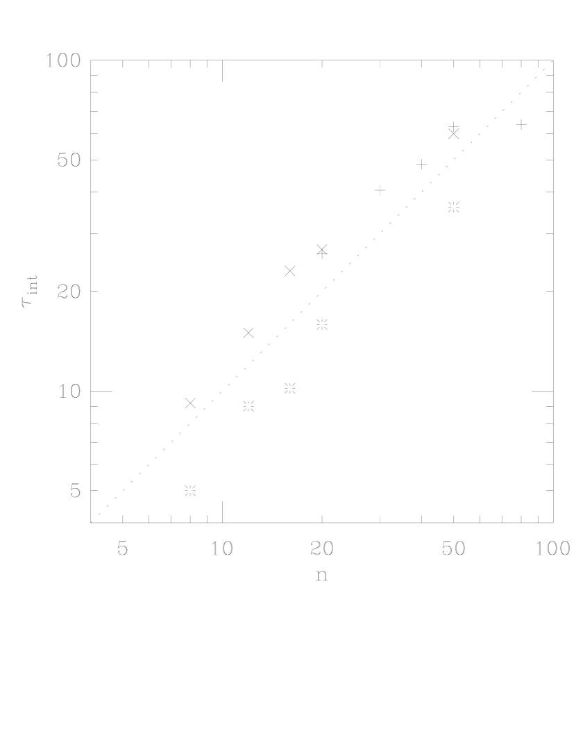
Figure 5: Integrated autocorrelation time of the plaquette, measured in sweeps, versus the number of bosonic fields. The dotted line shows $\tau_{int}=n$ to guid the eye. Crosses stand for a $4^{4}$ lattice, plusses for a $4^{3}\times 16$ lattice, both under a local update of the bosonic fields. Stars stand for a $4^{3}\times 16$ lattice, under a global heatbath of the bosonic fields. Simulations at $\beta=0,K=0.215$ without Metropolis test.

We first varied the number $n$ of bosonic fields, while keeping $\beta=0$ and $K=0.215$. Our data is shown by $\times$ and $+$ in Fig. 5, for a $4^{4}$ and $4^{3}\times 16$ lattice respectively. Independently of the volume, we get $\tau_{int}\sim 1.3n$. On the other hand, if we freeze the bosonic fields, updates of the gauge fields decorrelate the plaquette in ${\cal O}(1)$ sweep. The situation thus appears identical to the Hermitian case. Our explanation then [5] was that the slow dynamics were entirely caused by the bosonic fields, and that the autocorrelation time for the whole system was simply $\max_{k}\xi_{k}^{z}$, where $\xi_{k}$ is the $\phi_{k}$ correlation length and $z\sim 2$ the dynamic critical exponent. This scenario explained all our data. Here we test that scenario by applying a global heatbath at each sweep to each $\phi_{k}$. Namely we update the bosonic fields by the assignment $\phi_{k}\longleftarrow(D-z_{k})^{-1}\chi_{k}$, where $\chi_{k}$ is an independent Gaussian vector. While costly, this kind of updating should reduce the autocorrelation time of the bosonic dynamics, and thus of the whole system, to ${\cal O}(1)$ sweep. To our surprise, our measurements, shown by $\star$’s in Fig. 5, indicate that $\tau_{int}$ still grows linearly with $n$, and is only reduced by a factor $\sim 2$ compared to a local update. This is clearly caused by the coupling of all bosonic fields to each other, through the gauge field.

5.2 Toy model

To understand this phenomenon better, we consider a toy model of $n$ scalar complex variables $\tilde{\phi_{k}}$, and one scalar (complex or real) variable $x$, with action

$$S_{toy}=\sum_{k=1}^{n}|(x-z_{k})\tilde{\phi_{k}}|^{2}$$ (54)

The single variable $x$ thus plays the role of the Dirac operator $D$, and represents all the gauge degrees of freedom, while the $\tilde{\phi_{k}}$’s represent all the bosonic fields. The zeroes $\{z_{k}\}$ are the same as in eq.(8).

Consider Monte Carlo updates of this toy model, where the $\tilde{\phi_{k}}$’s are updated by a heatbath, and $x$ by over-relaxation. Namely, at each sweep:

$$\tilde{\phi_{k}}\longleftarrow\frac{1}{x-z_{k}}\tilde{\chi_{k}}$$ (55)

$$x\longleftarrow\frac{2\sum_{k}z_{k}|\tilde{\phi_{k}}|^{2}}{\sum_{k}|\tilde{\phi_{k}}|^{2}}-x$$ (56)

Substituting $(\ref{update_toy1})$ into $(\ref{update_toy2})$ gives

$$x_{new}-x=-2\frac{\sum_{k}\frac{1}{\bar{x}-\bar{z}_{k}}|\tilde{\chi_{k}}|^{2}}{\sum_{k}\frac{1}{|x-z_{k}|^{2}}|\tilde{\chi_{k}}|^{2}}$$ (57)

Since $|\tilde{\chi_{k}}|^{2}\sim 1$, one notices that the numerator above is $\sim-1/x$. On the other hand, since $|x-z_{k}|$ is bounded from above ($x$ must stay inside ${\partial\cal S}$), the denominator is bounded from below by some constant times $n$. The step size of the $x$ updates will therefore decrease like $1/n$, and the autocorrelation time increase like $n$, in spite of the heatbath on the $\tilde{\phi_{k}}$’s.

This analysis carries through whether $x$ is complex or real. There is a difference however, in the minimum distance $min_{k}|x-z_{k}|$. If $x$ is complex, it will stay most of the time well inside the domain ${\partial\cal S}$, and will only approach one of the zeroes $z_{k}$ occasionally. But if $x$ is real, which corresponds to the Hermitian algorithm, $x$ will always be near one of the zeroes $z_{k}$, because they all lie a distance $\sim 1/\sqrt{\epsilon}$ from the real axis, at intervals $\sim 1/n$. Therefore we should expect an additional slowing down $\sim 1/\sqrt{\epsilon}$ in this case, whereas the choice of “$K$” has little effect in the non-Hermitian case. These expectations are fully confirmed by numerical simulations of our toy model.

Going back to our original QCD action, we now understand why a global heatbath of the bosonic fields fails to decorrelate the gauge fields. We also expect another advantage of the non-Hermitian formulation: only a few modes of the gauge field, those with eigenvalues near ${\partial\cal S}$, will suffer additional slowing down (beyond a factor $n$) as $K$ approaches $K_{c}$; in the Hermitian formulation, all modes will slow down as $n/\sqrt{\epsilon}$. Unfortunately, we have not found any way to accelerate the dynamics in either case, even in our toy model.

5.3 Cost of the simulation

Since we now have a reasonable understanding of the Metropolis acceptance and of the dynamics without the Metropolis test, we can see the effect of the one on the other, and then estimate the total cost of the algorithm per independent configuration.

Denote by $W_{i}$ the value of our observable (the plaquette) at the beginning of trajectory $i$, and by $W_{i}^{\prime}$ the value for the candidate configuration proposed to the Metropolis test at the end of trajectory $i$. Then the probability distribution for $W_{i+1}$ is

$$P(W_{i+1})=P_{acc}\delta(W_{i}^{\prime})+(1-P_{acc})\delta(W_{i})$$ (58)

Assume for simplicity that $<W>=<W^{\prime}>=0$. The autocorrelation of $W$ will then be

$$\frac{<W_{i+1}W_{i}>}{<W>^{2}}=<P_{acc}>\frac{<W_{i}^{\prime}W_{i}>}{<W>^{2}}+(1-<P_{acc}>)$$ (59)

where we neglected correlations between $W_{i}^{\prime}$ and $P_{acc}$. Calling $\tau$ and $\tau_{0}$ the autocorrelation time with and without Metropolis respectively, we obtain

$$e^{-1/\tau}=<P_{acc}>e^{-m/\tau_{0}}+1-<P_{acc}>$$ (60)

or

$$\tau=\frac{-1}{\log(1-<P_{acc}>(1-e^{-m/\tau_{0}}))}$$ (61)

for a trajectory of $m$ sweeps. Note that $\tau_{0}$ is measured in sweeps and $\tau$ in trajectories. Folding into (61) our ansatz for $<P_{acc}>$ (eq. (53)), and using our empirical result $\tau_{0}\sim 1.3n$, we obtain in Fig. 4 the autocorrelation time as a function of n, for lattices of sizes 4, 8, 16, 32, at $\beta=0$ and $K=0.215$, with $m=10$. The behavior will be qualitatively similar for other choices of parameters. The Monte Carlo data shown in Fig. 6 was obtained on a $4^{4}$ lattice, and is roughly compatible with eq.(61).

The operation count of the algorithm is about $6n$ matrix-vector multiplications by the Dirac operator $D$ per sweep. Therefore we can estimate the total cost of our algorithm to produce an independent configuration, measured in multiplications by $D$ per lattice site, as a function of the number of fields or the Metropolis acceptance. This is shown in Figs. 7 and 8 respectively, for lattices of size $L=4$ to $32$. Fig. 7 shows, as expected, that the optimal number of bosonic fields grows logarithmically with the volume. The minimum work per site varies by a factor $<4$ going from $L=4$ to $32$. Recall that in HMC, the work per site is expected to grow like $L$, so it would increase by a factor 8 under the same change of volume. The asymptotic advantage of our algorithm thus translates into a slim factor $\sim 2$ for reasonable lattice sizes. Fig. 8 gives the useful hint that the acceptance should be kept high, $70-80\%$, but that the optimum is fairly broad. This high acceptance justifies a posteriori our neglect of the overhead due to the linear solver in the Metropolis test, since the number of iterations necessary is then ${\cal O}(1)$ (see Tables 1 and 2). It is also clear from this Figure that the Metropolis test actually saves a lot of work: if one wanted to get quasi-exact results (ie. acceptance $\sim 1$) without it, one would pay a factor $>_{\sim}4$ penalty, caused by the necessary increase both in the number of bosonic fields and in the autocorrelation time. Finally, it is instructive to compute the error bound (50) at the optimal acceptance point, since it is the analogue of the parameter $\delta$ of the original Lüscher proposal [1]: we get $\sim 1.4\%$ or $0.01\%$, for lattices of size 4 or 16; when the error becomes that small, it becomes most efficient to make the algorithm exact.

5.4 Scaling

The scaling of the number of bosonic fields and of the total complexity with the volume and the quark mass has already been discussed in [9]. Our analysis confirms these earlier estimates.

$\bullet$ As the volume $V$ increases, the number $n$ of bosonic fields should grow like $\log V$. This is a consequence of the exponential convergence of the polynomial approximation used (eq.(50)), and is clearly necessary to keep a constant Metropolis acceptance (eq.(53)). Since the work per sweep is proportional to $nV$, and the autocorrelation time to $n$, the work per independent configuration grows like $V(\log V)^{2}$. This is a slower growth than Hybrid Monte Carlo which requires work $\sim V^{5/4}$. But this is more of an academic than a practical advantage, as discussed above.

$\bullet$ As the quark mass $m_{q}$ decreases, the number of fields $n$ must grow like $m_{q}^{-1}$. This can be derived from eq.(50) or (53), using $m_{q}\propto 1-K/K_{c}$, which applies for small quark masses. The work per sweep is proportional to $n$. The autocorrelation time behavior is less clear. We expect that the autocorrelation behaves like $\tau\sim nm_{q}^{-\alpha}$, since $m_{q}$ enters in the effective mass term of each harmonic piece of the action $S_{b}$ (eq. 8), and since a factor $n$ comes from the autocorrelation of the gauge fields alone (remember the toy model in section 5.2). Our toy model does not say anything about local $\phi$ updates, so to determine $\alpha$ our main argument comes from MC data. From an exploratory simulation on a $4^{4}$ lattice at $\beta=0$ (see Table 6) we obtained that $\alpha$ is near $1$. This is only indicative, because the dependence of $\alpha$ with the volume and the coupling has yet to be explored.

K	$(1-K/K_{c})$	n	$\tau_{int}$	Work
0.215	0.14	14	5	4200
0.230	0.08	36	10	21600

Table 6: Exploratory measurement of the integrated autocorrelation time $\tau_{int}$ of the plaquette at $\beta=0$ on a $4^{4}$ lattice. The autocorrelation time is in units of trajectory. A trajectory is made of 10 sweeps. The degree of the polynomial is chosen to minimize the work. Each measurement is taken from a sample of 200000 sweeps.

Another interesting exploratory comparison was made between local and global heat-bath (see Table 7) without Metropolis test at $\beta=0$ on a $4^{3}\times 16$ lattice with fixed number of fields. We have measured the integrated autocorrelation of the plaquette for two quark masses. From the data in Table 7 it is clear that the exponent $\alpha$ is much lower for the global heat-bath, as expected from global algorithms. Of cource, the cost of a global heath-bath is prohibitive, because the matrix $(D-z_{k})$ has to be inverted for each boson field $\phi_{k}$. These simulations indicate that accelerating the boson fields using a cheaper algorithm than the global heat-bath could improve the dynamics substantially.

K	$(1-K/K_{c})$	n	$\tau_{int}$
			local HB+OR	global HB
0.215	0.14	20	26	16
0.230	0.08	20	65	22
0.240	0.04	20	150	?

Table 7: Exploratory measurement of the integrated autocorrelation time $\tau_{int}$ of the plaquette at $\beta=0$ on a $4^{3}\times 16$ lattice, for different quark masses and for local and global update of the boson fields. The degree of the polynomial is the same for all runs. The simulation is performed without Metropolis test. The autocorrelation time is in units of sweeps.

6 Conclusion

We have presented an alternative algorithm to HMC for simulating dynamical quarks in lattice QCD. This algorithm is based on a local bosonic action. A non-hermitian polynomial approximation of the inverse of the quark matrix is used to define the local bosonic action. The addition of a global Metropolis test corrects the systematic errors. The overhead of the correction test is minimal. Even-odd preconditioning can also be used improving the approximation by at least a factor of two. Its implementation is trivial.

This algorithm is exact for any choice of the polynomial approximation. No critical tuning of the approximation parameters is needed. Only the efficiency of the algorithm, which can be monitored, will be affected by the choice of parameters. The cost of the algorithm increases with the volume $V$ of the lattice as $V(\log V)^{2}$ and with the inverse of the quark mass $m_{q}$ as $\frac{n^{2}}{m_{q}^{\alpha}}\sim\frac{1}{m_{q}^{2+\alpha}}$ with $\alpha\simeq 1$. This compares favorably with the scaling of HMC.

Further extensions of this algorithm can be explored. In particular, non-local preconditioning techniques can cheaply be used because the inverse of the preconditioning matrix is not needed, contrary to HMC. A second possibility is to accelerate the dynamics of the boson fields, using non-local algorithms cheaper than a global heat-bath (for example multi-grid). A direct acceleration of the gauge fields is still an open problem.

Acknowledgments

We would like to thank the group of M. Lüscher for discussions and for allowing access to part of their documentation. We thank F.Jegerlehner for his help during the first stage of the project and B. Jegerlehner for helpfull discussions. Finally, we thank A. Boriçi and S. Solomon for useful suggestions and the SIC of the EPFL together with the support team of the Cray-T3D.

Appendix: Proof of eq.(49)

Detailed balance requires $<e^{-\Delta E}>=1$, so that $<(\Delta E)^{2}>\simeq 2<\Delta E>$. We assume that the distribution of $\Delta E$ is Gaussian. Let $x=\Delta E$ be a Gaussian distributed variable with variance $\sigma^{2}\simeq 2\bar{x}$. Its distribution is

$$P(x)=\frac{1}{\sigma\sqrt{2}\pi}\exp\left(-\frac{(x-\bar{x})^{2}}{2\sigma^{2}}\right)$$

From the Metropolis acceptance probability $P_{acc}=\min(1,e^{-\Delta E})$ we obtain

$$<P_{acc}> =\int_{-\infty}^{0}dxP(x)+\int_{0}^{\infty}dxP(x)e^{-x}=$$

$$=\frac{1}{\sigma\sqrt{2}\pi}\left[\int_{-\infty}^{0}dxe^{-\frac{(x-\bar{x})^{2}}{2\sigma^{2}}}+\int_{0}^{\infty}dxe^{-\frac{x^{2}-2x(\bar{x}-\sigma^{2})+\bar{x}^{2}}{2\sigma^{2}}}\right]=$$

$$=\frac{1}{\sigma\sqrt{2}\pi}\left[\int_{-\infty}^{-\bar{x}}dye^{\frac{-y^{2}}{2\sigma^{2}}}+\int_{-\bar{x}+\sigma^{2}}^{\infty}dye^{\frac{-y^{2}}{2\sigma^{2}}}e^{-\bar{x}+\sigma^{2}/2}\right]$$

Using the fact that $-\bar{x}+\sigma^{2}\simeq\bar{x}$ and $-\bar{x}+\sigma^{2}/2\simeq 0$ we obtain

$$<P_{acc}>\simeq \sqrt{\frac{2}{\pi}}\frac{1}{\sigma}\int_{\bar{x}}^{\infty}dye^{\frac{-y^{2}}{2\sigma^{2}}}=$$

$$=\frac{2}{\sqrt{\pi}}\int_{\frac{\bar{x}}{\sigma\sqrt{2}}}^{\infty}dte^{-t^{2}}=erfc\left(\frac{\bar{x}}{\sigma\sqrt{2}}\right)=erfc\left(\sqrt{\frac{<(\Delta E)^{2}>}{8}}\right)$$

Figure 1: Work per independent configuration as $K$ is varied. Dotted lines indicate the gain due to even-odd preconditioning. The abscissa is proportional to $m_{q}$ in the range of $K$ chosen. The work is measured in applications of the Dirac operator per site. The lattice size is $4^{4}$.

Figure 2: Metropolis acceptance as a function of the number of bosonic fields. The dotted line is our 1-parameter ansatz eq.(49).

Figure 3: Same as Fig.2, for a different value of $K$. The fit parameter $f$ (eq.(49)) is unchanged from Fig.2.

Figure 4: Same as Fig.2, for a different volume. The fit parameter $f$ (eq.(49)) is unchanged from Fig.2.

Figure 6: Integrated autocorrelation time given by our ansatz (58) as a function of the number of fields, measured in trajectories, for lattices of size $L=4,8,16,32$ from left to right. The Monte Carlo results also shown have been obtained for $L=4$.

Figure 7: Work per independent configuration versus the number of bosonic fields, for lattices of size $L=4,8,16,32$ from left to right. The work is measured in applications of the Dirac operator $D$ per site.

Figure 8: Same as Fig. 7, as a function of the Metropolis acceptance.

References

- [1] M.Lüscher, Nucl.Phys. B 418 (1994) 637
- [2] M.Peardon, Nucl. Phys B. (Proc. Suppl.) 42 (1995) 891
- [3] B.Bunk, K.Jansen, B.Jegerlehner, M.Lüscher, H.Simma and R.Sommer, Nucl. Phys. B (Proc. Suppl.) 42 (1995) 49
- [4] B.Jegerlehner, Nucl. Phys. B (Proc. Suppl.) 42 (1995) 879
- [5] C.Alexandrou, A.Borrelli, Ph. de Forcrand, A.Galli and F.Jegerlehner, Nucl. Phys. B 456 (1995) 296
- [6] A. Boriçi, Ph. de Forcrand, Nucl.Phys. B 454 (1995) 645
-
[7]
B. Jegerlehner, MPI-PHT-95-119, hep-lat/9512001
K. Jansen, B. Jegerlehner, C. Liu, hep-lat/9512018 - [8] I. Montvay, DESY 95-192, hep-lat/9510042
-
[9]
Ph. de Forcrand, IPS-95-24, hep-lat/9509082
A. Boriçi, Ph. de Forcrand, IPS-95-23, hep-lat/9509080 - [10] A. Frommer, V. Hannemann, B. Nockel, T. Lippert and K. Schilling, Int. J. Mod. Phys. C5 (1994) 1073
- [11] F.R.Brown and T.J.Woch, Phys. Rev. Lett. 58 (1987) 2394
- [12] R.Gupta at al., Phys. Rev. D 40 (1989) 2072