Asymptotic Scaling in theTwo-Dimensional $SU(3)$ $\sigma$-Modelat Correlation Length $4\times 10^{5}$

Abstract

We carry out a high-precision simulation of the two-dimensional $SU(3)$ principal chiral model at correlation lengths $\xi$ up to $\approx\!4\times 10^{5}$, using a multi-grid Monte Carlo (MGMC) algorithm. We extrapolate the finite-volume Monte Carlo data to infinite volume using finite-size-scaling theory, and we discuss carefully the systematic and statistical errors in this extrapolation. We then compare the extrapolated data to the renormalization-group predictions. For $\xi\mathrel{\hbox to0.0pt{\lower 3.0pt\hbox{$\mathchar 536\relax$}\hss}\raise 2.0pt\hbox{$\mathchar 318\relax$}}10^{3}$ we observe good asymptotic scaling in the bare coupling; at $\xi\approx 4\times 10^{5}$ the nonperturbative constant is within 2–3% of its predicted limiting value.

PACS number(s): 11.10.Gh, 11.15.Ha, 12.38.Gc, 05.70.Jk

A key tenet of modern elementary-particle physics is the asymptotic freedom of four-dimensional nonabelian gauge theories [1]. However, the nonperturbative validity of asymptotic freedom has been questioned [2]; and numerical studies of lattice gauge theory have thus far failed to detect asymptotic scaling in the bare coupling [3]. Even in the simpler case of two-dimensional nonlinear $\sigma$-models [4], numerical simulations at correlation lengths $\xi\sim 10$–100 have often shown discrepancies of order 10–50% from asymptotic scaling. In a recent paper [5] we employed a finite-size-scaling extrapolation method [6, 7, 8, 9] to carry simulations in the $O(3)$ $\sigma$-model to correlation lengths $\xi\approx 10^{5}$; the discrepancy from asymptotic scaling decreased from $\approx\!25\%$ to $\approx\!4\%$. In the present Letter we apply a similar technique to the $SU(3)$ principal chiral model, reaching correlation lengths $\xi\approx 4\times 10^{5}$ with errors $\mathrel{\hbox to0.0pt{\lower 3.0pt\hbox{$\mathchar 536\relax$}\hss}\raise 2.0pt\hbox{$\mathchar 316\relax$}}2\%$. For $\xi\mathrel{\hbox to0.0pt{\lower 3.0pt\hbox{$\mathchar 536\relax$}\hss}\raise 2.0pt\hbox{$\mathchar 318\relax$}}10^{3}$ we observe good asymptotic scaling in the bare parameter $\beta$; moreover, at $\xi\approx 4\times 10^{5}$ the nonperturbative ratio $\xi_{observed}/\xi_{theor,3-loop}$ is within 2–3% of the predicted limiting value.

We study the lattice $\sigma$-model taking values in the group $SU(N)$, with nearest-neighbor action ${\cal H}(U)=-\beta\sum\mathop{\rm Re}\nolimits\mathop{\rm tr}\nolimits(U_{x}^{\dagger}\,U_{y})$. Perturbative renormalization-group computations predict that the infinite-volume correlation lengths $\xi^{(exp)}$ and $\xi^{(2)}$ [10] behave as

$$\xi^{\#}(\beta)\;=\;C_{\xi^{\#}}\,e^{4\pi\beta/N}\,\left({4\pi\beta\over N}\right)^{\!-1/2}\,\left[1+{a_{1}\over\beta}+{a_{2}\over\beta^{2}}+\cdots\right]$$ (1)

as $\beta\to\infty$. Three-loop perturbation theory yields [12]

$$a_{1} = -0.121019N+0.725848N^{-1}-1.178097N^{-3}\;.$$ (2)

The nonperturbative constant $C_{\xi^{(exp)}}$ has been computed using the thermodynamic Bethe Ansatz [13]:

$$C_{\xi^{(exp)}}\;=\;{\sqrt{e}\over 16\sqrt{\pi}}\,{\pi/N\over\sin(\pi/N)}\,\exp\!\left(-\pi{N^{2}-2\over 2N^{2}}\right)\;.$$ (3)

The nonperturbative constant $C_{\xi^{(2)}}$ is unknown, but Monte Carlo studies indicate that $C_{\xi^{(2)}}/C_{\xi^{(exp)}}$ lies between $\approx\!0.985$ and 1 for all $N\geq 2$ [14]; for $N=3$ it is $0.987\pm 0.002$ [12]. Monte Carlo studies [16, 17, 18, 12] of the $SU(3)$ model up to $\xi\approx 35$ have failed to observe asymptotic scaling (1); the discrepancy from (1)–(3) is of order 10–20%.

Our extrapolation method [8] is based on the finite-size-scaling (FSS) Ansatz

$${{\cal O}(\beta,sL)\over{\cal O}(\beta,L)}\;=\;F_{{\cal O}}\Bigl{(}\xi(\beta,L)/L\,;\,s\Bigr{)}\,+\,O\Bigl{(}\xi^{-\omega},L^{-\omega}\Bigr{)}\;,$$ (4)

where ${\cal O}$ is any long-distance observable, $s$ is a fixed scale factor (here $s=2$), $L$ is the linear lattice size, $F_{{\cal O}}$ is a universal function, and $\omega$ is a correction-to-scaling exponent. We make Monte Carlo runs at numerous pairs $(\beta,L)$ and $(\beta,sL)$; we then plot ${\cal O}(\beta,sL)/{\cal O}(\beta,L)$ versus $\xi(\beta,L)/L$, using those points satisfying both $\xi(\beta,L)\geq$ some value $\xi_{min}$ and $L\geq$ some value $L_{min}$. If all these points fall with good accuracy on a single curve, we choose a smooth fitting function $F_{{\cal O}}$. Then, using the functions $F_{\xi}$ and $F_{\cal O}$, we extrapolate the pair $(\xi,{\cal O})$ successively from $L\to sL\to s^{2}L\to\ldots\to\infty$. See [8] for how to calculate statistical error bars on the extrapolated values.

We have chosen to use functions $F_{{\cal O}}$ of the form

$$F_{\cal O}(x)\;=\;1+a_{1}e^{-1/x}+a_{2}e^{-2/x}+\ldots+a_{n}e^{-n/x}\;.$$ (5)

We increase $n$ until the $\chi^{2}$ of the fit becomes essentially constant; the resulting $\chi^{2}$ value provides a check on the systematic errors arising from corrections to scaling and/or from inadequacies of the form (5). The discrepancies between the extrapolated values from different $L$ at the same $\beta$ can also be subjected to a $\chi^{2}$ test. Further details on the method can be found in [8, 5].

We simulated the two-dimensional $SU(3)$ $\sigma$-model using an $XY$-embedding multi-grid Monte Carlo (MGMC) algorithm [19]. We ran on lattices $L=8,16,32,64,$ $128,256$ at 184 different pairs $(\beta,L)$ in the range $1.65\leq\beta\leq 4.35$ (corresponding to $5\mathrel{\hbox to0.0pt{\lower 3.0pt\hbox{$\mathchar 536\relax$}\hss}\raise 2.0pt\hbox{$\mathchar 316\relax$}}\xi_{\infty}\mathrel{\hbox to0.0pt{\lower 3.0pt\hbox{$\mathchar 536\relax$}\hss}\raise 2.0pt\hbox{$\mathchar 316\relax$}}4\times 10^{5}$). Each run was between $4\times 10^{5}$ and $5\times 10^{6}$ iterations, and the total CPU time was one year on a Cray C-90 [20]. The raw data will appear in [21].

Our FSS data cover the range $0.08\mathrel{\hbox to0.0pt{\lower 3.0pt\hbox{$\mathchar 536\relax$}\hss}\raise 2.0pt\hbox{$\mathchar 316\relax$}}x\equiv\xi(L)/L\mathrel{\hbox to0.0pt{\lower 3.0pt\hbox{$\mathchar 536\relax$}\hss}\raise 2.0pt\hbox{$\mathchar 316\relax$}}1.12$, and we found tentatively that for ${\cal O}=\xi$ a thirteenth-order fit (5) is indicated: see Table 1. There are significant corrections to scaling in the regions $x\mathrel{\hbox to0.0pt{\lower 3.0pt\hbox{$\mathchar 536\relax$}\hss}\raise 2.0pt\hbox{$\mathchar 316\relax$}}0.84$ (resp. 0.64, 0.52, 0.14) when $L=8$ (resp. 16, 32, 64): see the deviations plotted in Figure 1. We therefore investigated systematically the $\chi^{2}$ of the fits, allowing different cuts in $x$ for different values of $L$: see again Table 1. A reasonable $\chi^{2}$ is obtained when $n\geq 13$ and $x_{min}\geq(0.80,0.70,0.60,0.14,0)$ for $L=(8,16,32,64,128)$. Our preferred fit is $n=13$ and $x_{min}=(\infty,0.90,0.65,0.14,0)$: see Figure 2, where we compare also with the perturbative prediction

$$F_{\xi}(x;s)\;=\;s\left[1\,-\,{aw_{0}\log s\over 2}x^{-2}\,-\,a^{2}\Biggl{(}{w_{1}\log s\over 2}+{w_{0}^{2}\log^{2}s\over 8}\Biggr{)}x^{-4}\,+\,O(x^{-6})\right]$$ (6)

valid for $x\gg 1$, where $a=2N/(N^{2}-1)$, $w_{0}=N/(8\pi)$ and $w_{1}=N^{2}/(128\pi^{2})$.

The extrapolated values $\xi_{\infty}^{(2)}$ from different lattice sizes at the same $\beta$ are consistent within statistical errors: only one of the 58 $\beta$ values has a $\chi^{2}$ too large at the 5% level; and summing all $\beta$ values we have $\chi^{2}=64.28$ (103 DF, level = 99.9%).

In Table 2 we show the extrapolated values $\xi_{\infty}^{(2)}$ from our preferred fit and some alternative fits. The deviations between the different fits (if larger than the statistical errors) can serve as a rough estimate of the remaining systematic errors due to corrections to scaling. The statistical errors in our preferred fit are of order 0.5% (resp. 0.9%, 1.1%, 1.3%, 1.5%) at $\xi_{\infty}\approx 10^{2}$ (resp. $10^{3}$, $10^{4}$, $10^{5}$, $4\times 10^{5}$), and the systematic errors are of the same order or smaller. The statistical errors at different $\beta$ are strongly positively correlated.

In Figure 3 (points $+$ and $\times$) we plot $\xi^{(2)}_{\infty,estimate\,(\infty,0.90,0.65)}$ divided by the two-loop and three-loop predictions (1)–(3) for $\xi^{(exp)}$. The discrepancy from three-loop asymptotic scaling, which is $\approx 13\%$ at $\beta=2.0$ ($\xi_{\infty}\approx 25$), decreases to 2–3% at $\beta=4.35$ ($\xi_{\infty}\approx 3.7\times 10^{5}$). For $\beta\mathrel{\hbox to0.0pt{\lower 3.0pt\hbox{$\mathchar 536\relax$}\hss}\raise 2.0pt\hbox{$\mathchar 318\relax$}}2.2$ ($\xi_{\infty}\mathrel{\hbox to0.0pt{\lower 3.0pt\hbox{$\mathchar 536\relax$}\hss}\raise 2.0pt\hbox{$\mathchar 318\relax$}}60$) our data are consistent with convergence to a limiting value $C_{\xi^{(2)}}/C_{\xi^{(exp)}}\approx 0.99$–1 with the expected $1/\beta^{2}$ corrections.

We can also try an “improved expansion parameter” [22, 12] based on the energy $E=N^{-1}\langle\mathop{\rm Re}\nolimits\mathop{\rm tr}\nolimits(U_{0}^{\dagger}\,U_{1})\rangle$. First we invert the perturbative expansion [12]

$$E(\beta)\;=\;1\,-\,{N^{2}-1\over 4N\beta}\,\left[1\,+\,{N^{2}-2\over 16N\beta}\,+\,{0.0756-0.0634\,{N^{2}}+0.01743\,{N^{4}}\over{N^{2}}\beta^{2}}\,+\,O(1/\beta^{3})\right]$$ (7)

and substitute into (1); this gives a prediction for $\xi$ as a function of $1-E$. For $E$ we use the value measured on the largest lattice (which is usually $L=128$); the statistical errors and finite-size corrections on $E$ are less than $5\times 10^{-4}$, and they induce an error less than $0.85\%$ on the predicted $\xi_{\infty}$ (less than 0.55% for $\beta\geq 2.2$). The corresponding observed/predicted ratios are also shown in Figure 3 (points $\Box$ and $\Diamond$). The “improved” 3-loop prediction is extremely flat, and again indicates a limiting value $\approx 0.99$.

Further discussion of the conceptual basis of our analysis can be found in [5]. Details of this work, including an analysis of the susceptibility $\chi$, will appear elsewhere [21].

A.P. would like to thank NYU for hospitality while some of this work was being carried out. These computations were performed on the Cray C-90 at the Pittsburgh Supercomputing Center and on the IBM SP2 cluster at the Cornell Theory Center. The authors’ research was supported by NSF grants DMS-9200719 and PHY-9520978.

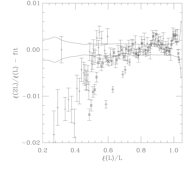
Figure 1: Deviation of points from fit to $F_{\xi}$ with $s=2$, $n=13$, $x_{min}=(\infty,\infty,\infty,0.14,0)$. Symbols indicate $L=8$ (+––$\tiny\vdash$$\tiny\dashv$), 16 ($\times$$\tiny\times$$\tiny\times$$\tiny\times$$\tiny\times$), 32 ($+$). Error bars are one standard deviation. Curves near zero indicate statistical error bars ($\pm$ one standard deviation) on the function $F_{\xi}(x)$.

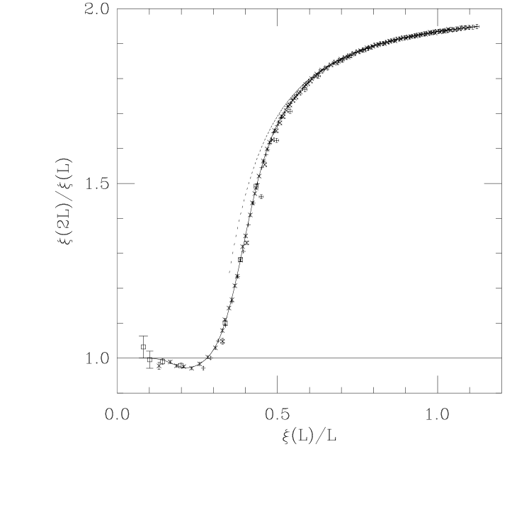
Figure 2: $\xi(\beta,2L)/\xi(\beta,L)$ versus $\xi(\beta,L)/L$. Symbols indicate $L=8$ (+––$\tiny\vdash$$\tiny\dashv$), 16 ($\times$$\tiny\times$$\tiny\times$$\tiny\times$$\tiny\times$), 32 ($+$), 64 ($\times$), 128 ($\Box$). Error bars are one standard deviation. Solid curve is a thirteenth-order fit in (5), with $x_{min}=(\infty,0.90,0.65,0.14,0)$ for $L=(8,16,32,64,128)$. Dashed curve is the perturbative prediction (6).

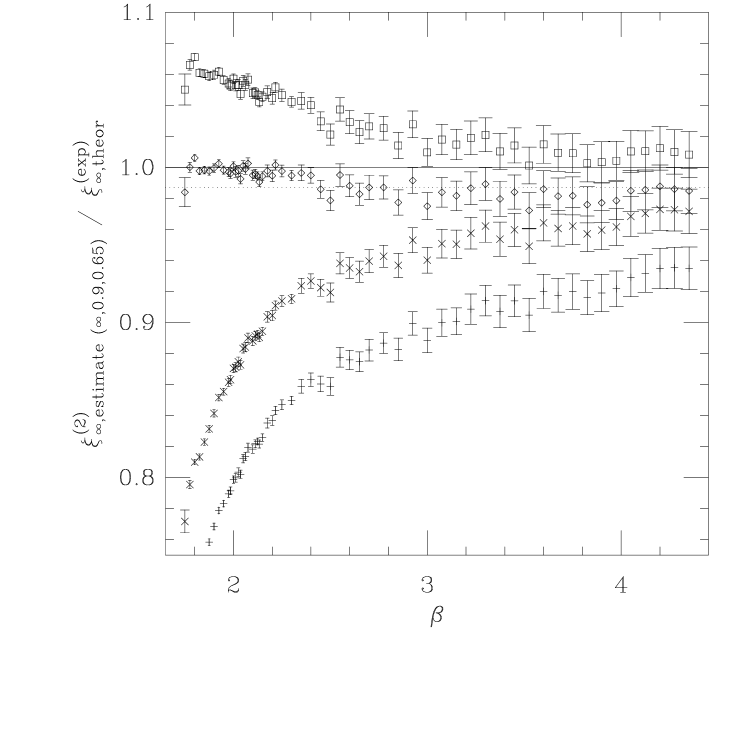
Figure 3: $\xi^{(2)}_{\infty,estimate\,(\infty,0.90,0.65)}/\xi^{(exp)}_{\infty,theor}$ versus $\beta$. Error bars are one standard deviation (statistical error only). There are four versions of $\xi^{(exp)}_{\infty,theor}$: standard perturbation theory in $1/\beta$ gives points $+$ (2-loop) and $\times$ (3-loop); “improved” perturbation theory in $1-E$ gives points $\Box$ (2-loop) and $\Diamond$ (3-loop). Dotted line is the Monte Carlo prediction $C_{\xi^{(2)}}/C_{\xi^{(exp)}}=0.987\pm 0.002$ [12].

$x_{min}$	$n=11$	$n=12$	$n=13$	$n=14$	$n=15$
(0.50,0.40,0)	180 718.80	179 626.60	178 560.20	177 558.60	176 558.30
	3.99 0.0%	3.50 0.0%	3.15 0.0%	3.16 0.0%	3.17 0.0%
($\infty$,0.40,0)	154 673.80	153 566.30	152 533.00	151 532.10	150 531.80
	4.38 0.0%	3.70 0.0%	3.51 0.0%	3.52 0.0%	3.55 0.0%
($\infty$,$\infty$,0)	108 236.00	107 172.40	106 154.80	105 154.70	104 153.40
	2.19 0.0%	1.61 0.0%	1.46 0.1%	1.47 0.1%	1.48 0.1%
(0.70,0.55,0.45)	162 288.30	161 219.20	160 183.00	159 182.50	158 182.30
	1.78 0.0%	1.36 0.2%	1.14 10.3%	1.15 9.8%	1.15 9.0%
(0.75,0.60,0.50)	150 222.40	149 172.20	148 129.90	147 129.80	146 129.80
	1.48 0.0%	1.16 9.4%	0.88 85.6%	0.88 84.3%	0.89 82.9%
(0.80,0.70,0.60)	129 173.90	128 135.00	127 96.30	126 96.28	125 94.31
	1.35 0.5%	1.05 32.0%	0.76 98.1%	0.76 97.7%	0.75 98.1%
(0.95,0.85,0.60)	111 150.30	110 107.20	109 77.62	108 77.62	107 75.67
	1.35 0.8%	0.97 55.8%	0.71 99.0%	0.72 98.8%	0.71 99.1%
(1.00,0.90,0.60)	105 139.20	104 100.90	103 70.74	102 70.73	101 67.50
	1.33 1.4%	0.97 56.7%	0.69 99.4%	0.69 99.2%	0.67 99.6%
($\infty$,0.90,0.65)	92 130.00	91 77.01	90 60.85	89 58.66	88 58.31
	1.41 0.6%	0.85 85.2%	0.68 99.2%	0.66 99.5%	0.66 99.4%
($\infty$,$\infty$,0.65)	78 96.09	77 56.51	76 49.55	75 46.63	74 45.94
	1.23 8.1%	0.73 96.2%	0.65 99.2%	0.62 99.6%	0.62 99.6%
($\infty$,$\infty$,$\infty$)	52 55.85	51 25.23	50 25.17	49 24.11	48 24.10
	1.07 33.2%	0.49 99.9%	0.50 99.9%	0.49 99.9%	0.50 99.8%

Table 1: Degrees of freedom (DF), $\chi^{2}$, $\chi^{2}$/DF and confidence level for the $n^{th}$-order fit (5) of $\xi(\beta,2L)/\xi(\beta,L)$ versus $\xi(\beta,L)/L$. The indicated $x_{min}$ values apply to $L=8,16,32$, respectively; we always take $x_{min}=0.14,0$ for $L=64,128$. Our preferred fit is shown in italics; other good fits are shown in sans-serif; bad fits are shown in roman.

$x_{min}$	1.80		2.00		2.20		2.40		2.60		2.85		3.00		3.15
(0.70,0.55,0.45)	10.455 (	0.022)	24.903 (	0.066)	57.13 (	0.17)	129.68 (	0.41)	290.5 (	1.0)	794.9 (	3.2)	1460 (	6)	2687 (	11)
(0.75,0.60,0.50)	10.454 (	0.022)	24.886 (	0.071)	57.50 (	0.18)	130.83 (	0.43)	293.0 (	1.1)	801.7 (	3.4)	1473 (	6)	2709 (	12)
(0.80,0.70,0.60)	10.450 (	0.021)	24.875 (	0.073)	57.41 (	0.22)	130.93 (	0.64)	293.6 (	1.6)	805.9 (	5.0)	1482 (	9)	2727 (	17)
(0.95,0.85,0.60)	10.451 (	0.021)	24.870 (	0.071)	57.40 (	0.21)	130.93 (	0.63)	293.7 (	1.6)	806.6 (	6.1)	1483 (	12)	2749 (	25)
(1.00,0.90,0.60)	10.450 (	0.022)	24.872 (	0.069)	57.40 (	0.21)	130.94 (	0.63)	293.6 (	1.6)	806.8 (	5.9)	1484 (	12)	2749 (	25)
($\infty$,0.90,0.65)	10.446 (	0.022)	24.859 (	0.072)	57.40 (	0.21)	131.00 (	0.66)	295.2 (	2.1)	809.6 (	6.7)	1489 (	13)	2761 (	27)
($\infty$,$\infty$,0.65)	10.447 (	0.022)	24.863 (	0.074)	57.40 (	0.22)	131.01 (	0.66)	295.0 (	2.1)	809.7 (	6.9)	1487 (	14)	2759 (	28)
($\infty$,$\infty$,$\infty$)	10.454 (	0.022)	24.881 (	0.074)	57.39 (	0.22)	130.78 (	0.66)	295.6 (	2.3)	812.7 (	9.8)	1482 (	22)	2777 (	49)

$x_{min}$	3.30		3.45		3.60		3.75		3.90		4.05		4.20		4.35
(0.70,0.55,0.45)	4957 (	23)	9117 (	46)	16780 (	92)	30959 (	182)	56766 (	362)	105205 (	707)	196197 (	1396)	360864 (	2792)
(0.75,0.60,0.50)	4995 (	24)	9199 (	47)	16938 (	93)	31258 (	185)	57265 (	366)	106093 (	736)	197949 (	1419)	363905 (	2880)
(0.80,0.70,0.60)	5032 (	32)	9268 (	62)	17066 (	118)	31492 (	239)	57687 (	456)	106807 (	878)	199117 (	1690)	366159 (	3309)
(0.95,0.85,0.60)	5109 (	49)	9411 (	92)	17359 (	178)	32059 (	346)	58748 (	650)	108781 (	1237)	202868 (	2360)	372553 (	4392)
(1.0,0.90,0.60)	5110 (	51)	9365 (	99)	17299 (	196)	31816 (	372)	58308 (	702)	107789 (	1312)	200994 (	2493)	369579 (	4697)
($\infty$,0.90,0.65)	5132 (	55)	9407 (	105)	17377 (	208)	31908 (	398)	58594 (	766)	108952 (	1452)	201796 (	2817)	371706 (	5457)
($\infty$,$\infty$,0.65)	5125 (	55)	9391 (	110)	17389 (	229)	32008 (	463)	58804 (	941)	109440 (	1886)	204587 (	3779)	376704 (	7722)
($\infty$,$\infty$,$\infty$)	5063 (	102)	9295 (	217)	16991 (	447)	30912 (	903)	55976 (	1828)	104740 (	3678)	192664 (	7358)	359299 (	14787)

Table 2: Estimated correlation lengths $\xi_{\infty}^{(2)}$ as a function of $\beta$, from various extrapolations. Error bar is one standard deviation (statistical errors only). All extrapolations use $s=2$ and $n=13$. The indicated $x_{min}$ values apply to $L=8,16,32$, respectively; we always take $x_{min}=0.14,0$ for $L=64,128$. Our preferred fit is shown in italic; other good fits are shown in sans-serif; bad fits are shown in roman.

References

- [1] M. Creutz, Quarks, Gluons, and Lattices (Cambridge Univ. Press, New York, 1983); H.J. Rothe, Lattice Gauge Theories: An Introduction (World Scientific, Singapore, 1992).
- [2] A. Patrascioiu, Phys. Rev. Lett. 54, 1192 (1985); A. Patrascioiu and E. Seiler, Max-Planck-Institut preprint MPI-Ph/91-88 (1991); Nucl. Phys. B (Proc. Suppl.) 30, 184 (1993); Phys. Rev. Lett. 74, 1920, 1924 (1995).
- [3] UKQCD Collaboration (S.P. Booth et al.), Nucl. Phys. B 394, 509 (1993); A. Ukawa, Nucl. Phys. B (Proc. Suppl.) 30, 3 (1993), section 6.2; G.S. Bali and K. Schilling, Phys. Rev. D47, 661 (1993); K.M. Bitar et al., hep-lat/9602010.
- [4] A.M. Polyakov, Phys. Lett. B59, 79 (1975); E. Brézin and J. Zinn-Justin, Phys. Rev. B14, 3110 (1976); W.A. Bardeen, B.W. Lee and R.E. Shrock, Phys. Rev. D14, 985 (1976); J.B. Kogut, Rev. Mod. Phys. 51, 659 (1979), section VIII.C.
- [5] S. Caracciolo, R.G. Edwards, A. Pelissetto and A.D. Sokal, Phys. Rev. Lett. 75, 1891 (1995). See also A. Patrascioiu and E. Seiler, Phys. Rev. Lett. 76, 1178 (1996); S. Caracciolo, R.G. Edwards, A. Pelissetto and A.D. Sokal, Phys. Rev. Lett. 76, 1179 (1996).
- [6] M. Lüscher, P. Weisz and U. Wolff, Nucl. Phys. B359, 221 (1991).
- [7] J.-K. Kim, Phys. Rev. Lett. 70, 1735 (1993); Nucl. Phys. B (Proc. Suppl.) 34, 702 (1994); Phys. Rev. D50, 4663 (1994); Europhys. Lett. 28, 211 (1994); Phys. Lett. B345, 469 (1995).
- [8] S. Caracciolo, R.G. Edwards, S.J. Ferreira, A. Pelissetto and A.D. Sokal, Phys. Rev. Lett. 74, 2969 (1995).
- [9] See note 8 of reference [5] for further history of this method.
- [10] Here is the exponential correlation length (= inverse mass gap), and is the second-moment correlation length defined by (4.11)–(4.13) of Ref. [11]. Note that is well-defined in finite volume as well as in infinite volume; where necessary we write and , respectively. In this paper, without a superscript denotes .
- [11] S. Caracciolo, R.G. Edwards, A. Pelissetto and A.D. Sokal, Nucl. Phys. B403, 475 (1993).
- [12] P. Rossi and E. Vicari, Phys. Rev. D49, 1621, 6072 (1994); D50, 4718 (E) (1994).
- [13] J. Balog, S. Naik, F. Niedermayer and P. Weisz, Phys. Rev. Lett. 69, 873 (1992).
- [14] The principal chiral model is equivalent to the -vector model; and the expansion of the latter model, evaluated at , indicates that [15]. Monte Carlo data on the chiral model with can be found in [12].
- [15] H. Flyvbjerg, Nucl. Phys. B348, 714 (1991); P. Biscari, M. Campostrini and P. Rossi, Phys. Lett. B242, 225 (1990); S. Caracciolo and A. Pelissetto, in preparation.
- [16] E. Dagotto and J.B. Kogut, Nucl. Phys. B290[FS20], 451 (1987).
- [17] M. Hasenbusch and S. Meyer, Phys. Rev. Lett. 68, 435 (1992).
- [18] R.R. Horgan and I.T. Drummond, Phys. Lett. B327, 107 (1994).
- [19] G. Mana, T. Mendes, A. Pelissetto and A.D. Sokal, Dynamic critical behavior of multi-grid Monte Carlo for two-dimensional nonlinear -models, presented at the Lattice ’95 conference, hep-lat/9509030, Nucl. Phys. B (Proc. Suppl.) __, ___ (1996).
- [20] This is an “equivalent” CPU time; some runs on the smaller lattices were performed on an IBM SP2.
- [21] G. Mana, A. Pelissetto and A.D. Sokal, Multi-grid Monte Carlo via embedding. II. Two-dimensional principal chiral model, in preparation.
- [22] G. Martinelli, G. Parisi and R. Petronzio, Phys. Lett. B100, 485 (1981); S. Samuel, O. Martin and K. Moriarty, Phys. Lett. B153, 87 (1985); G.P. Lepage and P.B. Mackenzie, Phys. Rev. D48, 2250 (1993).