DAMTP 96-04

KL-TH 3/96

The Roughening Transition of the 3D Ising

Interface: A Monte Carlo Study

M. Hasenbusch,

DAMTP, Silver Street, Cambridge, CB3 9EW, England

S. Meyer and M. Pütz

Fachbereich Physik, Universität Kaiserslautern , Germany

We study the roughening transition of an interface in an Ising system on a 3D simple cubic lattice using a finite size scaling method. The particular method has recently been proposed and successfully tested for various solid on solid models. The basic idea is the matching of the renormalization-group-flow of the interface with that of the exactly solvable body centered cubic solid on solid model. We unambiguously confirm the Kosterlitz-Thouless nature of the roughening transition of the Ising interface. Our result for the inverse transition temperature $K_{R}=0.40754(5)$ is almost by two orders of magnitude more accurate than the estimate of Mon, Landau and Stauffer [9].

Key words: Ising model, roughening transition, Monte Carlo, finite size scaling, renormalization group.

1 Introduction

Interfaces play an essential role in many areas of science. In condensed matter physics, the most prominent examples are surfaces of liquids and solids. In 1951 Burton, Cabrera and Frank [1] pointed out that a phase transition may occur in the equilibrium structure of crystal surfaces. Such a phase transition from a smooth to a rough surface is called a roughening transition. They viewed a growing layer of a crystal as a two dimensional Ising model. The part of the layer occupied by atoms is represented by spin +1, while the vacancies are represented by spin -1. From the exact solution of the two-dimensional Ising model [2] one then infers the existence of a phase transition. However this picture of a crystal surface is very crude. Obviously in a real crystal surface there are more than just one single incomplete layer of atoms.

A better description of a crystal in equilibrium with its vapour is provided by the three-dimensional Ising model, where spin +1 represents a site occupied by an atom, while spin -1 represents a vacancy. The boundary conditions are chosen such that an interface between a region with most spins equal to +1 and a region with most spins equal to -1 is present. In 1973 Weeks et al. [3] performed a low temperature expansion for the width of an (001) interface in a three-dimensional Ising model on a simple cubic lattice with isotropic couplings. They obtained a roughening temperature $T_{R}=0.57\;\;T_{c}$, where $T_{c}$ is the temperature of the bulk phase transition, while the approximation of the interface by the two dimensional Ising model yields $T_{R}=0.503\;\;T_{c}$. The best known value for the inverse of the critical temperature of the three-dimensional Ising model on a simple cubic lattice is given by $\beta=0.2216546(10)$ [4].

A fairly good approximation of the Ising interface is given by the so called SOS (solid on solid) models. Neglecting overhangs of the interface and bubbles in the bulk, the variables of the two dimensional models give the height of the interface measured above some reference plane. A duality transformation exactly relates these models with two dimensional $XY$ models [5]. In contrast to the two-dimensional Ising model which undergoes a second-order phase transition, SOS models, as $XY$ models, are expected to undergo a Kosterlitz-Touless (KT) phase transition [6].

The important question is whether overhangs of the interface and bubbles in the bulk-phases are irrelevant for the critical behaviour of the interface in the Ising model and hence the roughening transition is of KT nature as it is the case for SOS models. Monte Carlo simulations of the interface in a three-dimensional Ising model have been performed in order to answer this question [7, 8, 9].

However, the numerical determination of the transition temperature and the confirmation of the KT nature of the phase transition has turned out to be extremely difficult. The reason for this problem can be found in the KT theory itself. At the roughening transition corrections are present that vanish logarithmically with the length scale. Therefore for all lattices sizes that can be simulated one is quite far away from the Gaussian fixed point that is the basis for the formulas used for fits in refs. [7, 8, 9]. In order to overcome this problem one has to take into account the logarithmic corrections in the analysis of the data [10].

However one can do even better. The body centered cubic solid on solid (BCSOS) model that was introduced by van Beijeren in 1977 [11] as a solid on solid approximation of an interface in an Ising model on a body centered cubic lattice on a (001) lattice plane is solved exactly. The BCSOS model is equivalent with one of the exactly solved vertex models [12, 13, 14]. The exact formula for the free energy and the correlation length proves the model to have a KT-type phase transition.

In [15, 16] it was proposed to match the renormalization group (RG)-flow of other SOS models and the Ising interface with that of the BCSOS model. The RG-flow is monitored by properly chosen block-observables on finite lattices. In order to determine the roughening temperature of an SOS model or the Ising interface one has to find the temperature where the values for the block-observables for the BCSOS model at the roughening temperature are reproduced.

This method has been successfully applied to the ASOS (absolute value SOS) model, the discrete Gaussian model and the dual of the standard $XY$ model in 2 dimensions [15]. Preliminary results were also obtained for the Ising interface [16].

In the present paper we improve the result of ref. [16] by drastically increasing the statistics for the Ising model as well as for the BCSOS model. The largest lattice size considered is increased from $64\times 64\times 27$ to $256\times 256\times 31$ allowing the direct matching of the Ising interface with the BCSOS model compared with the indirect approach via the ASOS model of ref. [16]. The high statistical accuracy needed for the matching method could be obtained in a moderate amount of CPU time (about two months on a workstation) due to the use of highly efficient cluster algorithms for the Ising interface [23] as well as for the BCSOS model [22].

This paper is organized as follows. In section 2 we define the models to be studied. We summarize exact results for the BCSOS model [12, 13, 14] relevant to our study. We briefly discuss the RG-flow diagram of the KT phase-transition. In section 3 we describe the matching method. We give particular emphasis to the special problems arising in the case of the Ising interface. In section 4 we discuss our numerical results. A comparison with previous Monte Carlo studies is presented in section 5. In section 6 we give our conclusions and an outlook.

2 The models

We consider an Ising model on a simple cubic lattice with extension $L$ in x- and y-direction and with extension $D$ in z-direction. For reasons given by the algorithm we shall only consider odd values of $D$. We have chosen the convention that the z-coordinate of the lattice points takes the half-integer values $z=-D/2\;...\;D/2$. The Ising model is defined by the partition function

$$Z=\sum_{s_{i}=\pm 1}\exp(-K^{I}H)\;,$$ (1)

where the classical Hamiltonian is given by

$$H=-\sum_{<ij>}J_{<ij>}s_{i}s_{j}\;,$$ (2)

where the summation is taken over all nearest neighbour pairs $<ij>$ on the lattice, and $K_{I}=\frac{1}{k_{B}T}$ is the normalized inverse temperature. In x- and y-direction we consider periodic boundary conditions. In order to create an interface we apply anti-periodic boundary conditions in the remaining z-direction. Anti-periodic boundary conditions are defined by $J_{<ij>}=-1$ for bonds $<ij>$ connecting the lowermost and uppermost plane of the lattice, while all other nearest neighbour pairs keep $J_{<ij>}=1$.

The ASOS model is the solid on solid approximation of an interface in an Ising system on a simple cubic lattice on a (001) lattice plane. It is defined by the partition function

$$Z=\sum_{h_{i}}\exp(-K^{ASOS}\sum_{<i,j>}|h_{i}-h_{j}|)\;,$$ (3)

where $h_{i}$ is integer-valued and the summation is taken over the nearest neighbour pairs of a 2D square lattice. At low temperatures the Ising interface and the ASOS model are related by $2K^{I}=K^{ASOS}$.

In the case of the BCSOS model the two-dimensional lattice splits in two sub-lattices like a checker board. In the original formulation, on one of the sub-lattices the spins takes integer values, whereas the spins on the other sublattice take half-integer values. We adopt a different convention: spins on “odd” lattice sites take values of the form $2n+(1/2)$, and spins on “even” sites are of the form $2n-(1/2)$, $n$ integer. As a consequence, the effective distribution for block spins (= averages over blocks) will be centered around integer values (instead of half integer values), and the average of the lowest energy configurations take integer values like it is the case for the ASOS models defined above. The partition function of the BCSOS model can be expressed as

$$Z=\sum_{h}\exp(-K^{S}\sum_{[i,k]}|h_{i}-h_{k}|)\;,$$ (4)

where $i$ and $k$ are next to nearest neighbours. Nearest neighbour spins $h_{i}$ and $h_{j}$ obey the constraint $|h_{i}-h_{j}|=1$. Van Beijeren [11] has shown that the configurations of the BCSOS model are in one-to-one correspondence to the configurations of the F model, which is a special six vertex model. The F model can be solved exactly with transfer matrix methods [12, 13, 14]. For our choice of the field variable the roughening coupling is given by

$$K_{R}^{S}=\frac{1}{2}\ln 2.$$

The critical behaviour of non-local quantities such as the correlation length $\xi$ is known and has the form predicted by KT theory [14].

The RG-flow of SOS models is well described by two parameters $\beta$ and $y$ [6]. The two dimensional Sine Gordon model is especially suited to discuss the flow of these parameters with the length scale, since this model contains $\beta$ and $y$ as bare parameters in its action. On the lattice it is given by the partition function

$$Z^{SG}=\int[\mbox{d}\phi]\;\exp\left(-\frac{1}{2\beta}\sum_{<i,j>}(\phi_{i}-\phi_{j})^{2}+y\sum_{i}\cos(2\pi\phi_{i})\right),$$ (5)

where the $\phi_{i}$ are real numbers.

For the continuum version of the model with a momentum cutoff one can derive the parameter flow under infinitesimal RG transformations [6]. It is given, to second order in perturbation theory, by

$$\dot{x}=-z^{2}\;,\;\;\;\;\;\;\;\;\;\;\;\;\dot{z}=-xz\;,$$ (6)

where $z=const\cdot y$ and $x=\pi\beta-2$. $const$ depends on the particular cutoff scheme used. The derivative is taken with respect to the logarithm of the cutoff scale. For large $x$, $z$ flows towards $z=0$. The large distance behaviour of the model is therefore the same as that of the massless Gaussian model. For small $x$, $z$ increases with increasing length scale. The theory is therefore massive. The critical trajectory separates these two regions in the coupling space. It ends at a Gaussian fixed point characterized by $x=0$ or $\beta=\frac{2}{\pi}$. On the critical trajectory the fugacity vanishes as

$$z(t)=\frac{1}{z_{0}^{-1}+t}\;,$$ (7)

where $t$ is the logarithm of the cutoff scale.

3 The matching method

In order to compare the RG-flows of the Ising interface and the BCSOS model we follow closely the method introduced in ref. [15]. This method is closely related to the finite size scaling methods proposed by Nightingale [19] and Binder [20]. No attempt is made to compute the RG-flow of the couplings explicitly, but rather the RG-flow is monitored by evaluating quantities that are primarily sensitive to the lowest frequency fluctuations on a finite lattice.

In order to separate the low frequency modes of the field a block-spin transformation [21] is used. Blocked systems of size $l\times l$ are considered. The size $B$ of a block (measured in units of the original lattice spacing) is then given by $B=L/l$, where $L$ is the linear size of the original lattice. For solid on solid models the block-spins are defined by

$$\phi_{\tilde{j}}=B^{-2}\sum_{j\in\tilde{j}}h_{j}\;,$$ (8)

where $\tilde{j}$ labels square blocks of a linear extension $B$. One should note that this linear blocking rule has the half-group property that the successive applications of two transformations with a scale-factor of $B$ have exactly the same effect as a single transformation with a scale-factor of $B^{2}$.

Since the position of the interface in the Ising system is not well defined on a microscopic level we have to look for a substitute of the blocking rule applied to the field of the SOS models. In the following we briefly discuss the solution of the problem proposed and applied to the study of interfaces in the rough phase in ref. [24].

First we have to ensure that the interface is not located at the $z=-D/2$ to $z=D/2$ boundary, in which case the definition of the blockspin discussed below would become meaningless. Therefore we locate the interface in the system in a crude fashion, which is done by searching for the z-slice with the smallest absolute value of the magnetisation. Then we redefine the $z$- coordinates such that the interface is located close to $z=0$. Now one can go ahead with the measurement of interface properties ignoring the periodicity of the lattice in z-direction.

The blocks considered have the full lattice extension D in z-direction and an extension $B$ in x- and y-direction. The interface position is defined inside a block by

$$\phi_{\tilde{i}}=\frac{M_{\tilde{i}}}{2mB^{2}}\;,$$ (9)

where $M_{\tilde{i}}$ is the total magnetisation in the block $\tilde{i}$ and $m$ is the bulk magnetisation. This definition is motivated by the naive picture that above the interface the magnetisation takes uniformly the value $-m$ and below the value $m$.

One has to discuss to what extent the meaning of the above definition is spoiled by corrections to this simple picture. What are the effects of bulk fluctuations and overhangs of the interface? The fluctuations of the bulk magnetisation are given by the magnetic susceptibility $\chi$. The square of the fluctuations of $M_{\tilde{i}}$ induced by the bulk fluctuation is therefore given by $\sigma^{2}(M_{\tilde{i}})=DB^{2}\chi$ and the resulting fluctuations of $\phi_{\tilde{i}}$ induced by bulk fluctuations is given by

$$\sigma^{2}_{b}(\phi_{\tilde{i}})=\frac{1}{4}\frac{D}{B^{2}}\frac{\chi}{m^{2}}\;.$$ (10)

As a consequence the larger the block size in x- and y-direction, the better the position of the interface is defined. However, when $D$ is sent to infinity for a fixed $B$, the position of the interface defined by eq. (9) becomes meaningless.

In ref. [23, 15] we proposed a radical solution to overcome the problem of bulk fluctuations completely. Before the position of the interface is determined all bubbles are removed. Technically this is accomplished by performing standard cluster-updates at $K=\infty$. Since the absolute value of the bulk magnetisation becomes 1 in this process the definition of the interface position is modified to

$$\bar{\phi}_{\tilde{i}}=\frac{\bar{M}_{\tilde{i}}}{2B^{2}}\;.$$ (11)

Overhangs of the interface are expected on a scale of the bulk correlation length $\xi_{b}$. Therefore we have to assume that the position of the interface only has a well defined meaning if the blocksize is large compared with the bulk correlation length $B>>\xi_{b}$. At the roughening transition this is however no severe restriction since $\xi_{b}\approx 0.3$.

Finally one should ensure that no additional interfaces are created spontaneously. Following ref. [25] the surface tension at $K^{I}=0.40$ is $\sigma=0.6721(1)$. This is certainly a lower bound for the surface tension at the roughening coupling to be found below. Therefore two additional interfaces are suppressed by at least a factor of $D^{2}\exp(-0.6721\times 2L^{2})$, which is certainly sufficient already for the smallest lattice size $L=32$ that we consider.

Now we define suitable observables for the blocked systems discussed above. Motivated by the perturbation theory of the Sine-Gordon model two types of observables are chosen: such that are “sensitive” to the flow of the kinetic term (flow of $K$), and such that are sensitive to the fugacity (periodic perturbation of a massless Gaussian model). For the first type of observables we choose

$$A_{1}=\langle(\phi_{\tilde{i}}-\phi_{\tilde{j}})^{2}\rangle\;,$$ (12)

where $\tilde{i}$ and $\tilde{j}$ are nearest neighbours on the block lattice, and

$$A_{2}=\langle(\phi_{\tilde{i}}-\phi_{\tilde{k}})^{2}\rangle\;,$$ (13)

where $\tilde{i}$ and $\tilde{k}$ are next to nearest neighbours. Note that these quantities are only defined for $l>1$. As a monitor for the fugacity we take the following set of quantities (defined for $l=1,2,4$):

$$A_{3} = \langle\cos(2\pi\phi_{\tilde{i}})\rangle$$

$$A_{4} = \langle\cos(2\cdot 2\pi\phi_{\tilde{i}})\rangle$$

$$A_{5} = \langle\cos(3\cdot 2\pi\phi_{\tilde{i}})\rangle$$ (14)

3.1 Determination of the roughening coupling

As discussed in ref. [15] there are two parameters which have to be adjusted in order to match the RG flow of the Ising interface with that of the critical BCSOS model: The coupling $K^{I}$ of the Ising interface and in addition the ratio $b=B^{I}/B^{S}=L^{I}/L^{S}$ of the lattice sizes (and hence the block sizes) of the Ising model and the BCSOS model. A $b\neq 1$ is needed to compensate for the different starting points of the two models on the critical RG-trajectory. In ref. [15, 16] $b=3.3(3)$ was obtained.

For the proper values of the roughening coupling $K^{I}_{R}$ and the matching constant $b$ observables of the Ising interface and the BCSOS model match like

$$A_{i,l}^{I}(b\;B,K^{I}_{R})=A_{i,l}^{S}(B,K^{S}_{R})+O(B^{-\omega})\;,$$ (15)

where $i$ indicates the observable and $l$ the size of the blocked lattice. The $O(B^{-\omega})$ corrections are due to irrelevant operators. $\omega$ is the correction to scaling exponent. The perturbation theory of the Sine-Gordon model suggests $\omega=2$.

In order to obtain a numerical estimate for the roughening coupling $K^{I}_{R}$ of the Ising model and the matching factor $b$ for a given lattice size $L^{S}$ of the BCSOS model we required that the equation above is exactly fulfilled for two block observables.

In the following we considered the pairs $(A_{1,l},A_{3,l})$ and $(A_{2,l},A_{3,l})$ for $l=2$ and $l=4$. Replacing $A_{3,l}$ by $A_{4,l}$ or $A_{5,l}$ leads to statistically poorer results.

We solved the system of two equations for the two observables $A_{i,l}$ and $A_{j,l}$ numerically by first computing the $K^{I}_{i,l}(b)$ and $K^{I}_{j,l}(b)$ that solve the single equations for a given value of $b$. The intersection of the two curves $K^{I}_{i,l}(b)$ and $K^{I}_{j,l}(b)$ gives us then the solution of the system of two equations. For an illustration of this method see figures 5 and 6 of ref. [15].

In [15] it was demonstrated, that the corrections to scaling for the observables $A_{1}$ and $A_{2}$ for SOS models are similar to those in the massless continuous Gaussian model. Therefore we considered the “improved” observable $D_{1}$ which is defined as follows:

$$D_{1}(L)=\frac{A_{1}^{(0)}(\infty)}{A_{1}^{(0)}(L)}A_{1}(L)$$ (16)

$A_{1}^{(0)}$ is computed for the massless Gaussian model defined by

$$Z_{0}=\int\prod_{x}d\psi_{x}\exp(-\frac{1}{2}\sum_{<x,y>}(\psi_{x}-\psi_{y})^{2})$$ (17)

An improved quantity $D_{2}$ is defined analogously. Explicit results for $A_{1}^{(0)}$ and $A_{2}^{(0)}$ are given in table 4 of ref. [15].

Obviously this modification does not affect the large $L$ behaviour since $A_{1}^{(0)}(L)=A_{1}^{(0)}(\infty)+O(L^{-2})$. In the following we will see that the results for our largest lattice sizes are virtually unaffected by this kind of improvement. However the benefit for the smaller lattices will be clearly visible.

4 Discussion of the numerical results

First we simulated the BCSOS model at the roughening coupling $K_{R}=\frac{1}{2}\ln 2$ on square lattices of the size $L\times L$ with periodic boundary conditions imposed. We considered lattices with sizes ranging from $L=8$ up to $L=96$. The loop algorithm of Evertz, Marcu and Lana [22] enabled us to reduce the statistical error of the BCSOS data compared with those given in [15] by a factor of about 5. We performed $4\cdot 10^{6}$ measurements throughout, except for $L=96$, where $3\cdot 10^{6}$ measurements were performed. The number of loop-updates per measurement was 10 for $L=8$ up to 35 for $L=96$. This number was chosen such that the integrated autocorrelation times in units of measurements were about 1. These simulations took about 81 hours of CPU time on a IBM RISC System/6000 Modell 590 (66 Mhz) in total. The results for $l=4$ for the critical BCSOS model are presented in figures 2 to 6. The numbers for the $A$’s can be obtained from the authors on request.

Next we performed the simulations of the Ising model at the best known value $K_{R}=0.4074$ [16] for the roughening coupling. We used the modified cluster algorithm introduced in [23]. For a discussion of the algorithm see also ref. [24]. The expectation values for $K^{I}$ in the neighbourhood of the simulation point are then obtained by re-weighting [26].

First of all we had to ensure that our results are not spoiled by a to small extension in z-direction. Obviously the thickness of the lattice has to be large compared to the width of the interface itself. It turns out that this requirement can be easily fulfilled since the width of the interface at $K_{R}$ is smaller than 1 for the lattice size we will consider in the following [7, 23, 9, 24].

In [23, 24, 25] the dependence of interface properties on the extension of the lattice in z-direction was carefully checked. For couplings close to $K_{R}$ and lattice sizes $L\leq 256$ it turned out that for about $D>10$ no dependence on $D$ can be detected within the obtained accuracy.

We performed an additional check for $L=128$. We compared the interface width without bubbles for $D=15$ and $D=31$. We obtain $W_{0}^{2}=0.64647(25)$ for $D=15$ and $W_{0}^{2}=0.64658(33)$ for $D=31$. The definition of $W_{0}^{2}$ is given below.

Therefore we regard the extension $D=31$ which we used throughout in the following simulations as perfectly safe.

Per measurement we performed 5 H-updates and 5 I-updates and in addition one Metropolis sweep. Remember that H and I refer to reflections at half-integer and integer z-values respectively. The number of updates per sweep was again chosen such that the integrated autocorrelation times in units of measurements are smaller than 1. The number of measurements was 100000 for most of the lattice sizes. For $L=48$, $192$ and $L=256$ we performed $93500$, $113000$ and $72500$ measurements respectively. The total amount of CPU time used for the Ising simulations was about 63 days on an IBM RISC System/6000 Modell 590 (66 Mhz).

4.1 The interface width

Before discussing the results of the matching analysis let us briefly study the behaviour of the surface width, which was the basis of the Monte Carlo study of ref. [9]. Following ref. [9] a normalized magnetization gradient is defined as

$$\rho(z)=\frac{1}{2m_{b}L^{2}}[M(z+1/2)-M(z-1/2)]\;,$$ (18)

where $m_{b}$ is the bulk magnetization and $M$ the total magnetization of a z-slize of the lattice. Now the interface width is given by

$$W^{2}=\langle\;\sum_{z}\rho(z)z^{2}-\left(\sum_{z}\rho(z)\rho(z)z\right)^{2}\;\rangle\;.$$ (19)

We computed the interface width for the original configurations ($W^{2}$) and after removing the bubbles ($W_{0}^{2}$). In the rough phase of the Ising interface or an SOS model the surface width behaves like

$$W^{2}=const+\frac{1}{2\pi\beta_{eff}}\ln L$$ (20)

for sufficiently large $L$. $\beta_{eff}$ is determined by the point where the RG-trajectory hits the $x$ axis in the $KT$ flow diagram. Therefore the slope of the curve at the roughening transition should be given by $1/\pi^{2}$. However it was pointed out in refs. [15, 10] that at the roughening transition corrections to this asymptotic behaviour die out proportional to the fugacity (7) i.e. only proportional to the inverse of the logarithm of $L$. Hence these corrections cannot be neglected even for quite large lattice sizes.

To check this anticipated behaviour we have plotted the surface thickness for the BCSOS model and the Ising interface with bubbles and bubbles removed in figure 1. For comparison two straight lines with slope $1/\pi^{2}$ are given. It turns out that even when our largest lattice sizes are considered the slope is by about $10\%$ larger than the asymptotic one. Using therefore eq. (20) with the slope $1/\pi^{2}$ as criterion to determine the roughening point leads to a considerable under-estimation of the roughening temperature. Going to enormous lattice sizes such as $L=960$ does not help that much to overcome the problem since the corrections die out only logarithmically in $L$.

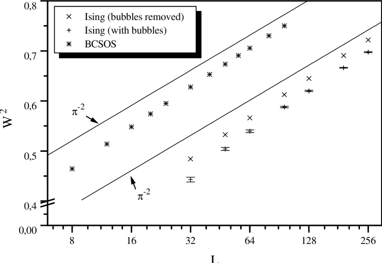
Figure 1: Squared interface width $W^{2}$ plotted versus the lattice size $L$

4.2 Matching results

For the determination of the roughening temperature and the matching factor using the matching method we have considered the four pairs of observables $(A_{1,2},A_{3,2})$, $(A_{2,2},A_{3,2})$, $(A_{1,4},A_{3,4})$ and $(A_{2,4},A_{3,4})$. In order to check the effect of removing the bubbles and the improvement by the continuous Gaussian model on our results we performed the whole analysis for the following four different choices of the observables:
iii) The bubbles being removed from the bulk phases, using the improved $D_{1}$ and $D_{2}$.
iii) The bubbles being removed from the bulk phases, using $A_{1}$ and $A_{2}$.
iii) Not removing the bubbles, using the improved $D_{1}$ and $D_{2}$.
iv) Not removing the bubbles, using $A_{1}$ and $A_{2}$.

In all cases the statistical errors of the estimates for the roughening coupling and the matching factor were computed from a Jackknife analysis put on top of the whole matching procedure.

The results for the roughening coupling $K_{R}$ for the Ising interface based on i) and ii) are summarized in table 1. Using the improved quantities $D_{1}$ and $D_{2}$ the results are consistent within two standard deviations starting from $L=96$ for $l=2$ as well as $l=4$. For our largest lattice size $L=256$ the difference of the results when using the unimproved observables $A_{1}$ and $A_{2}$ rather than $D_{1}$ and $D_{2}$ is smaller than the statistical error. However looking at the results obtained from $L=32$ and $L=48$ makes clear that a major part of the corrections to scaling is eliminated by using $D_{1}$ and $D_{2}$ instead of $A_{1}$ and $A_{2}$.

Table 1: Results for the roughening coupling obtained from matching for different values of $L$ and $l=2,4$. For the matching $A_{3,l}$ together with either $A_{1,l}$ , $D_{1,l}$ , $A_{2,l}$ or $D_{2,l}$ is used. The bubbles in the Ising system are removed before the measurement.

$L$	$l$	$A_{1}$	$D_{1}$	$A_{2}$	$D_{2}$
32	2	0.40602(15)	0.40727(14)	0.40657(16)	0.40831(21)
48	2	0.40648(16)	0.40716(16)	0.40678(17)	0.40760(21)
64	2	0.40675(14)	0.40722(14)	0.40692(15)	0.40735(18)
96	2	0.40719(14)	0.40741(15)	0.40727(16)	0.40745(17)
128	2	0.40733(15)	0.40748(16)	0.40734(19)	0.40748(21)
192	2	0.40762(14)	0.40768(14)	0.40762(15)	0.40766(16)
256	2	0.40748(14)	0.40751(14)	0.40762(16)	0.40765(16)
32	4	0.40529(10)	0.40678(9)	0.40589(10)	0.40740(10)
48	4	0.40610(9)	0.40709(8)	0.40647(9)	0.40748(9)
64	4	0.40649(8)	0.40728(8)	0.40677(9)	0.40750(9)
96	4	0.40702(8)	0.40745(8)	0.40717(8)	0.40754(9)
128	4	0.40727(7)	0.40752(7)	0.40733(8)	0.40755(9)
192	4	0.40753(7)	0.40766(7)	0.40754(7)	0.40764(8)
256	4	0.40738(7)	0.40745(7)	0.40741(7)	0.40746(7)

In table 2 we present the results for the matching factor $b$ based on i) and ii). The observations are analogous to those for the roughening coupling.

Table 2: Results for matching parameter $b$ for different values of $(L)$ and $(l=2,4)$. For the matching $A_{3,l}$ together with either $A_{1,l}$ , $D_{1,l}$ , $A_{2,l}$ or $D_{2,l}$ is used. Bubbles are removed from the Ising configurations.

$L$	$l$	$A_{1}$	$D_{1}$	$A_{2}$	$D_{2}$
32	2	2.12(4)	2.68(5)	2.346(6)	3.14(11)
48	2	2.30(8)	2.74(12)	2.49(10)	3.05(16)
64	2	2.54(11)	2.92(12)	2.68(11)	3.02(16)
96	2	2.60(14)	2.84(18)	2.69(17)	2.88(20)
128	2	2.85(19)	3.05(23)	2.86(24)	3.05(29)
192	2	2.74(24)	2.82(27)	2.73(26)	2.80(28)
256	2	3.08(33)	3.15(35)	3.45(44)	3.54(48)
32	4	1.751(10)	2.048(11)	1.864(13)	2.194(18)
48	4	2.062(18)	2.419(22)	2.191(24)	2.548(28)
64	4	2.311(26)	2.703(32)	2.442(33)	2.816(42)
96	4	2.550(41)	2.87(6)	2.66(5)	2.95(7)
128	4	2.68(6)	2.91(7)	2.73(7)	2.94(8)
192	4	2.81(9)	2.96(10)	2.82(10)	2.94(11)
256	4	3.05(11)	3.16(12)	3.10(13)	3.19(13)

For a block-size $B\geq 32$ the results obtained from iii) and iv) are consitent within error-bars with those obtained from i) and ii) . We therefore skip a detailed discussion of these results.

Following the above discussion we regard the results for $K_{R}$ and $b$ obtained from i) as the least affected by systematical errors. Therefore we take the weighted average of the results of i) (i.e. the $D_{1}$ and $D_{2}$ columns of table 1 and 2) for $l=2$, $L\geq 96$ and $l=4$, $L\geq 128$ as our final result.

We obtain $K_{R}=0.40754(5)$ and $b=2.97(7)$. Computing the error-estimate we have assumed that values obtained from the same simulation but from a different pair of observables are strongly correlated.

As an additional check of universality we have plotted all observables $A_{i}$ considered for the critical BCSOS model as well as the Ising interface at $K_{R}=0.40754(5)$ as a function of $L$ and $L/b$ respectively in figures 2-6.

In figure 2 the observables $A_{14}$ and $D_{14}$ are plotted. The figure shows nicely the improvement gained by replacing $A_{14}$ by $D_{14}$. While the curves of $A_{14}$ for the Ising interface and the BCSOS model are only consistent for $L\leq 192$, the consistency extends down to at least $L=96$ when $D_{14}$ is considered. For $A_{24}$ and $D_{24}$ given in figure 3 this improvement is visible even more drastically.

In the case of $A_{34}$ plotted in figure 4 the matching of the curves within the statistical accuracy sets in for $L^{I}\geq 64$.

In figure 5 the observable $A_{44}$ is plotted. This observable was not used for the determination of $K_{R}$ and $b$. The fact that for $L^{I}\geq 96$ the curves of $A_{4,4}$ for the Ising interface and the BCSOS model fall on top of each other, strongly supports that the Ising interface and the BCSOS model have the same critical behaviour. For $L^{I}\geq 128$ also the curves of $A_{5,4}$ for the Ising interface and the BCSOS model become identical within error bars.

Similar observations hold for $l=1$ and $l=2$. (The correponding figures are not reproduced here.)

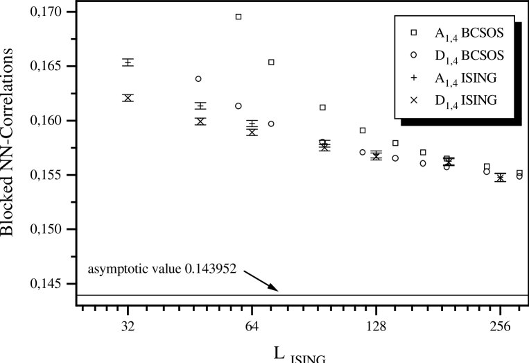
Figure 2: $A_{1,4}$ and $D_{1,4}$ at the roughening transition as a function of $L^{I}=b~{}L^{S}$ for the Ising interface as well as the BCSOS model

Figure 3: $A_{2,4}$ and $D_{2,4}$ at the roughening transition as a function of $L^{I}=b~{}L^{S}$ for the Ising interface as well as the BCSOS model

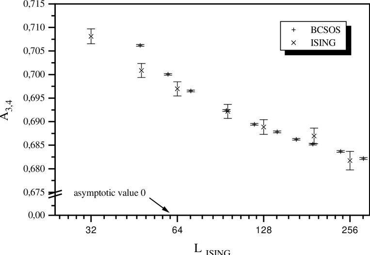
Figure 4: $A_{3,4}$ at the roughening transition as a function of $L^{I}=b~{}L^{S}$ for the Ising interface as well as the BCSOS model

Figure 5: $A_{4,4}$ at the roughening transition as a function of $L^{I}=b~{}L^{S}$ for the Ising interface as well as the BCSOS model

Figure 6: $A_{5,4}$ at the roughening transition as a function of $L^{I}=b~{}L^{S}$ for the Ising interface as well as the BCSOS model

The matching programme also allows to determine the nonuniversal constants appearing in formulas describing the divergence of observables near the roughening transition. The critical behaviour of the correlation length $\xi$ is described by [6]

$$\xi=A\;\exp(C\;\kappa^{-1/2})\;\;.$$ (21)

Along the lines of section 5.3 of ref. [15] we obtain $A^{I}=0.74(2)$ and $C^{I}=1.03(2)$ for the Ising interface.

5 Comparison with existing studies

Let us compare our result, $K_{R}=0.40754(5)$, with results obtained in previous Monte Carlo studies of the Ising interface.

We nicely confirm the value $K_{R}=0.4074(3)$ obtained by one of the present authors [16] using similar methods as used in the present paper.

In a large scale Monte Carlo simulation of lattices up to $960\times 960\times 26$ Mon, Landau and Stauffer [9] studied the behaviour of the interface width. They obtain $K_{R}^{I}=0.409(4)$.

Mon, Wansleben, Landau and Binder [8] determined the step free energy on lattices of size up to $96^{3}$. They give the estimate $T_{R}/T_{c}=0.54(2)$ which corresponds to $K_{R}=0.410(16)$.

Bürkner and Stauffer [7] obtained in their pioneering study $T_{R}/T_{c}=0.56(3)$ which corresponds to $K_{R}=0.396(22)$.

One should note that all these estimates are consistent within the quoted error-bars with our present result.

It is also interesting to compare the Ising interface results with those obtained in ref. [15] for the ASOS model, $K_{R}^{ASOS}=0.8061(3)$ and $b_{m}^{ASOS}=2.8(3)$. In the low temperature limit the ASOS coupling and that of the Ising model are related as $K^{I}=1/2K_{ASOS}$. At finite temperatures one expects that the bubbles and the overhangs disorder the Ising interface compared to the ASOS model. Hence one expects the roughening transition of the Ising interface to occur at a lower temperature as for the ASOS model and indeed $K_{R}^{I}-1/2K_{R}^{ASOS}=0.0044(2)$.

Such a shift was already predicted by low temperature expansions [27], $K_{R,LT}^{I}=0.404(12)$ and $K_{R,LT}^{ASOS}=0.787(24)$. However one should note that the difference of these two results is smaller than the given error-bars. The matching factors for the two models are equal within the quoted error-bars. The direct matching of the Ising interface with the ASOS model performed in ref. [16] gives the more precise result $b_{m}^{I}/b_{m}^{ASOS}=1.17(4)$ for this particular comparison.

6 Conclusion and outlook

Using the finite size scaling method of ref. [15] we unambigously demonstrated the KT-nature of the roughening transition in the (001) interface of the 3D Ising model. Our estimate for the inverse of the roughening temperature $K_{R}=0.40754(5)$ is almost by a factor of 100 more accurate then the best previously published value [9].

Previous studies have been mainly plagued by logarithmic corrections at the roughening transition. This problem has been overcome completely.

In addition the use of efficient, virtually slowing-down free, cluster algorithms for the BCSOS model [22] and the Ising interface [23, 24] allowed us to generate more than $10^{6}$ independent configurations in the case of the BCSOS model and about $10^{5}$ independent configurations for the Ising model for all lattice sizes using about 2 month of CPU time on an IBM RISC System/6000 Modell 590 (66 Mhz).

This high statistical accuracy can be further improved. First simply by using more CPU time and secondly by further improvements in the implementation of the algorithm.

Figure Captions

Fig.1
Squared interface width $W^{2}$ plotted versus the lattice size $L$

Fig.2
$A_{1,4}$ and $D_{1,4}$ at the roughening transition as a function of $L^{I}=b~{}L^{S}$ for the Ising interface as well as the BCSOS model

Fig.3
$A_{2,4}$ and $D_{2,4}$ at the roughening transition as a function of $L^{I}=b~{}L^{S}$ for the Ising interface as well as the BCSOS model

Fig.4
$A_{3,4}$ at the roughening transition as a function of $L^{I}=b~{}L^{S}$ for the Ising interface as well as the BCSOS model

Fig.5
$A_{4,4}$ at the roughening transition as a function of $L^{I}=b~{}L^{S}$ for the Ising interface as well as the BCSOS model

Fig.6
$A_{5,4}$ at the roughening transition as a function of $L^{I}=b~{}L^{S}$ for the Ising interface as well as the BCSOS model

References

- [1] W.K.Burton, N.Cabrera, F.C.Frank, Phil.Trans.Roy.Soc.(London) 243 A (1951) 299.
- [2] L.Onsager, Phys.Rev 65 (1944) 117.
- [3] J.D.Weeks, G.H.Gilmer and H.J Leamy, Phys.Rev.Lett. 31 (1973) 549.
- [4] H.W.J. Blöte, E. Luijten and J.R. Heringa, cond-mat/9509016, to be published in J.Phys.A.
- [5] R. Savit, Rev. Mod. Phys. 52 (1980) 453, and references therein.
-
[6]
To give only a few references:
J. M. Kosterlitz and D. J. Thouless, J.Phys.C 6 (1973) 1181. J. M. Kosterlitz, J.Phys.C 7 (1974) 1046. S.T.Chui and J.D.Weeks Phys.Rev.B 14 (1976) 4978; J.V.José, L.P.Kadanoff, S.Kirkpatrick and D.R.Nelson, Phys. Rev. B 16 (1977) 1217; T.Ohta and K.Kawasaki, Prog.Theor.Phys.60 (1978) 365 ; D.J.Amit, Y.Y. Goldschmidt and G.Grinstein, J.Phys.A 13 (1980) 585. H.van Beijeren and I.Nolden, The Roughening Transition, in Topics in Current Physics Vol. 43, W. Schommers and P. van Blankenhagen editors (Springer, 1987) p. 259; - [7] E.Bürkner and D.Stauffer, Z.Phys.B 53 (1983) 241.
- [8] K.K.Mon, S.Wansleben, D.P.Landau and K.Binder, Phys.Rev.Lett. 60 (1988) 708.
- [9] K.K.Mon, D.P.Landau and D.Stauffer, Phys.Rev.B 42 (1990) 545.
- [10] H.G. Evertz, M. Hasenbusch, M. Marcu, K. Pinn, Physica A 199 (1993) 31.
- [11] H.van Beijeren, Phys.Rev.Lett. 38 (1977) 993.
- [12] E.H.Lieb, Phys.Rev.162 (1967) 162.
- [13] E.H.Lieb and F.Y.Wu, in Phase Transitions and Critical Phenomena, C.Domb and N.S.Green editors, Vol.1 (Academic London) (1972).
- [14] R.J.Baxter, Exactly Solved Models in Statistical Mechanics , Academic Press (1982).
- [15] M. Hasenbusch, M. Marcu, K. Pinn, Physica A 208 (1994) 124.
- [16] M. Hasenbusch, PhD Thesis, Universität Kaiserslautern, 1992.
-
[17]
K.G.Wilson,
Physica 73 (1974) 119;
K.G.Wilson and J.Kogut,
Phys.Rep.C 12 (1974) 75 ,
and references therein. - [18] Phase transitions and Critical Phenomena, edited by C.Domb and M.S.Green (Academic, London) Vol.6 (1976).
- [19] M.P. Nightingale, Physica A 83 (1976) 561.
- [20] K.Binder: Monte Carlo Investigations of Phase Transitions and Critical Phenomena, in: C.Domb and M.S.Green (eds.): Phase Transitions and Critical Phenomena, Vol. 5b, Academic Press, New York, 1976.
- [21] L.P.Kadanoff, Physics 2 (1966) 263.
- [22] H.G.Evertz, M. Marcu, G. Lana, Phys.Rev.Lett. 70 (1993) 875.
- [23] M.Hasenbusch and S.Meyer, Phys.Rev.Lett. 66 (1991) 530.
- [24] M. Hasenbusch and K. Pinn, Physica A 192 (1993) 342.
- [25] M. Hasenbusch and K. Pinn, Physica A 203 (1994) 189.
- [26] R.H.Swendsen and A.M.Ferrenberg, Phys.Rev.Lett 61 (1988) 2635.
- [27] J.Adler, Phys.Rev.B 36 (1987) 2473.