The Lattice Schrödinger Functional and the
Background Field Effective Action

Abstract

We propose a new method that by using the lattice Schrödinger functional allows to investigate the effective action for external background fields in lattice gauge theories. We show that this method gives sensible results for the case of four-dimensional U(1) gauge theory in an external constant magnetic field.

BARI-TH 218/95

, and

1 Introduction

The Euclidean Schrödinger functional in Yang-Mills theories without matter fields is defined by

$${\mathcal{Z}}\left[A^{(f)},A^{(i)}\right]=\langle A^{(f)}|\exp(-HT){\mathcal{P}}|A^{(i)}\rangle\,,$$ (1)

where the operator ${\mathcal{P}}$ projects onto the physical states and $H$ is the pure gauge Yang-Mills Hamiltonian in the temporal gauge. $A^{a(i)}_{k}\left(\vec{x}\right)$ and $A^{a(f)}_{k}\left(\vec{x}\right)$ are classical gauge fields, and the state $|A\rangle$ is such that

$$\left\langle A|\Psi\right\rangle=\Psi(A)$$ (2)

for all wave functionals $\Psi(A)$. From Equation(1), inserting an orthonormal basis $\{|\Psi_{n}\rangle\}$ of gauge invariant energy eigenstates, it follows

$${\mathcal{Z}}\left[A^{(f)},A^{(i)}\right]=\sum_{n}\exp(-E_{n}T)\Psi_{n}\left(A^{(f)}\right)\Psi^{*}_{n}\left(A^{(i)}\right)\,,$$ (3)

where $E_{n}$ are the energy eigenvalues. Note that Eq.(3) implies that ${\mathcal{Z}}\left[A^{(f)},A^{(i)}\right]$ is invariant under arbitrary gauge transformations of the fields $A^{(f)}$ and $A^{(i)}$.

The authors of Refs.[1, 2] studied the Schrödinger functional in lattice gauge theories. It turns out that the Schrödinger functional has a well-defined continuum limit and, moreover, it is amenable to numerical simulations [2]. The lattice Schrödinger functional is given by

$${\mathcal{Z}}\left[U^{(f)},U^{(i)}\right]=\int{\mathcal{D}}U\exp(-S)\,.$$ (4)

In Equation(4) the action $S$ is the standard Wilson action modified to take into account the boundaries at $x_{4}=0$, and $x_{4}=T$ [2]:

$$S=\frac{1}{g^{2}}\sum_{x,\mu>\nu}w_{\mu\nu}(x)\text{Tr}\left[1-U_{\mu\nu}(x)\right]\,,$$ (5)

where the $w_{\mu\nu}(x)$’s are equal to $1/2$ for the spatial plaquettes at $x_{1}=0$ and $x_{1}=T$, otherwise they are equal to 1. Obviously, in Eq.(4) one integrates over the links $U_{\mu}(x)$ with the fixed boundary values

$$U(x)|_{x_{4}=0}=U^{(i)}\,,\quad U(x)|_{x_{4}=T}=U^{(f)}\,.$$ (6)

The external links $U^{(i)}$ and $U^{(f)}$ are the lattice implementation of the smooth classical boundary fields $A_{k}^{a(i)}(x)$ and $A_{k}^{a(f)}(x)$. It is worthwhile to stress that the functional Eq.(4) is invariant under arbitrary lattice gauge transformations of the boundary links. Moreover, we note that in the numerical simulations of the lattice Schödinger functional one can assume periodic boundary conditions in the spatial directions, while the periodicity in the time direction is lost if $U^{(i)}\neq U^{(f)}$.

The aim of the present paper is to investigate the lattice effective action for external background fields. Let us consider a static external background field $\vec{A}^{\text{ext}}(\vec{x})=\vec{A}_{a}^{\text{ext}}(\vec{x})\lambda_{a}/2$, where $\lambda_{a}/2$ are the generators of the SU(N) Lie algebra. On the lattice the dynamical variables are the links $U_{\mu}(x)$. The natural relation between the continuum gauge field and the corresponding lattice link is given by

$$U_{\mu}^{\text{ext}}(x)={\text{P}}\exp\left\{+iag\int_{0}^{1}dt\,A_{\mu}^{\text{ext}}(x+at{\hat{\mu}})\right\}$$ (7)

where P is the path-ordering operator. We can now define the lattice effective action for the background field $A_{\mu}^{\text{ext}}(\vec{x})$ by means of the lattice Schrödinger functional Eq.(4)as follows:

$$\Gamma\left[\vec{A}^{\text{ext}}\right]=-\frac{1}{T}\ln\left\{\frac{{\mathcal{Z}}[U^{\text{ext}}]}{{\mathcal{Z}}(0)}\right\}$$ (8)

where $T$ is the extension in the Euclidean time. In Equation(8) we define ${\mathcal{Z}}[U^{\text{ext}}]={\mathcal{Z}}[U^{\text{ext}},U^{\text{ext}}]$, and ${\mathcal{Z}}(0)$ means the lattice Schrödinger functional without external background field ($U_{\mu}^{\text{ext}}=1$). From the previous discussion it is clear that $\Gamma\left[\vec{A}^{\text{ext}}\right]$ is invariant for lattice gauge transformations of the external links $U_{\mu}^{\text{ext}}(\vec{x})$. In particular, if we consider background fields that give rise to constant field strength, then it is easy to show that $\Gamma\left[\vec{A}^{\text{ext}}\right]$ is proportional to the spatial volume $V$. In this case one is interested in the density of the effective action:

$$\varepsilon\left[\vec{A}^{\text{ext}}\right]=-\frac{1}{V\cdot T}\ln\left[\frac{{\mathcal{Z}}[U^{\text{ext}}]}{{\mathcal{Z}}(0)}\right]\,.$$ (9)

Note that our definition of the lattice effective action uses the lattice Schrödinger functional with the same boundary fields at $x_{4}=0$ and $x_{4}=T$. As a consequence we can glue the two hyperplanes $x_{0}=0$ and $x_{0}=T$ together. Thus, we end up in a lattice with periodic conditions in the time direction too. Therefore we have

$${\mathcal{Z}}[U^{\text{ext}}]=\int{\mathcal{D}}U\,\exp(-S)\,.$$ (10)

with the constraints

$$U_{\mu}(x)|_{x_{4}=0}=U_{\mu}^{\text{ext}}\,.$$ (11)

In other words the Schrödinger functional Eq.(10) is given by the standard partition function on a periodic lattice with a cold wall at $x_{4}=0$. Note that, due to the lacking of free boundaries, the action in Eq.(10) is now the familiar Wilson action

$$S=S_{W}=\frac{1}{g^{2}}\sum_{x,\mu>\nu}{\text{Tr}}\left[1-U_{\mu\nu}(x)\right]\,.$$ (12)

In the remainder of this paper we test our definition of lattice effective action in the case of the simplest lattice gauge theory, namely the U(1) compact pure gauge theory without matter fields.

2 U(1) effective action

It is known that for Wilson action on a four-dimensional lattice with periodic boundary conditions, the electric charge is confined for $\beta<\beta_{c}\simeq 1.01$, while for $\beta>\beta_{c}$ the gauge system is made of free photons. Moreover, the phase transition is triggered by the condensation of magnetic monopoles [3, 4, 5, 6]. In the seminal paper by DeGrand and Toussaint [4] it has been shown that external magnetic fields are sensitive to the lattice magnetic monopoles. In particular, it turns out that for strong coupling (in four dimensions) monopoles screen external magnetic fields, while for weak coupling the magnetic fields penetrates into the lattice. Thus it is worthwhile to investigate the lattice effective action for constant background magnetic fields. In the continuum the vector potential corresponding to a constant magnetic field along the $x_{3}$ direction is given by

$$A_{k}^{\text{ext}}(\vec{x})=\delta_{k,2}x_{1}B$$ (13)

in the Landau gauge. From Eq.(7) it follows

$$\begin{split}U_{2}^{\text{ext}}(x)=\exp\left[iagBx_{1}\right]=\cos(agBx_{1})+i\sin(agBx_{1})\,,\\ U^{\text{ext}}_{1}(x)=U^{\text{ext}}_{3}(x)=U^{\text{ext}}_{4}(x)=1\,.\end{split}$$ (14)

The periodic boundary conditions result in the quantization of the external magnetic field

$$a^{2}gB=\frac{2\pi}{L_{1}}n^{\text{ext}}$$ (15)

where $n^{\text{ext}}$ is an integer and $L_{1}$ is the lattice extension in the $x_{1}$ direction in lattice units. The action corresponding to the links (14) on a lattice of size $L_{1}L_{2}L_{3}L_{4}$ with periodic boundary conditions is readily evaluated:

$$S^{\text{ext}}=\beta\Omega\left[1-\cos(a^{2}gB)\right]$$ (16)

where $\beta=1/g^{2}$, and $\Omega=L_{1}L_{2}L_{3}L_{4}$ is the lattice volume. Note that in the naive continuum limit $S^{\text{ext}}$ reduces to $V\cdot T\,\frac{B^{2}}{2}$. Equation(16) shows that, in order to be close to the continuum limit on a finite lattice, we must require that $a^{2}gB\ll 1$. This in turn implies that $L_{1}\gg 1$. Moreover, in order to select the ground state contribution in the sum (3), we also need $L_{4}\gg 1$. As a consequence we performed our numerical simulations on lattices with size $L_{1}=64$, $L_{4}=32$ and $L_{2}=L_{3}=6,\,8,\,10$. We use the standard Metropolis algorithm to update gauge configurations. The links belonging to the time slice $x_{4}=0$ are frozen to the configuration (14). In addition we impose that the links at the spatial boundaries are fixed according to (14). In the continuum this condition amounts to the usual requirement that the fluctuations over the background field vanish at the infinity.

As a preliminary step, it is important to test the behaviour of the magnetic field. To this end we look at the field strength tensor for a given time slice. We define

$$F_{\mu\nu}(x_{4})=\sqrt{\beta}\,\left\langle\frac{1}{V}\sum_{\vec{x}}\sin\theta_{\mu\nu}(\vec{x},x_{4})\right\rangle$$ (17)

where $\theta_{\mu\nu}(\vec{x},x_{4})$ is the plaquette angle in the $(\mu,\nu)$ plane. Clearly for $x_{4}=0$ (or $x_{4}=L_{4}$ due to the periodic boundary conditions) we have

$$F_{12}(0)\equiv F_{12}^{\text{ext}}=\sqrt{\beta}\sin\left(\frac{2\pi}{L_{1}}n^{\text{ext}}\right)\,,$$ (18)

the other components of the field strength tensor being equal to zero. In Figures 1 and 2 we display $F_{\mu\nu}$ versus the Euclidean time $x_{4}$ for the $64\times 10^{2}\times 32$ lattice and $n^{\text{ext}}=2$. As expected, we find that only the component $F_{12}$ of the field strength tensor is present in our data. For $\beta<1$ the external magnetic field is shielded after a small penetration (Fig. 1). On the other hand, for $\beta>1$ (Fig. 2) the field penetrates indicating that the gauge system supports a long range magnetic field.

We now turn on the evaluation of the density of the effective action (9). We face with the problem of computing a partition function which is the exponential of an extensive quantity [7]. To avoid this problem we consider the derivative of $\varepsilon[\vec{A}^{\text{ext}}]$ with respect to $\beta$. We get

$$\varepsilon^{\prime}\left[\vec{A}^{\text{ext}}\right]=\frac{\partial\varepsilon\left[\vec{A}^{\text{ext}}\right]}{\partial\beta}=-\frac{1}{\Omega}\,\left[\frac{1}{Z[U^{\text{ext}}]}\frac{\partial Z[U^{\text{ext}}]}{\partial\beta}-\frac{1}{Z[0]}\frac{\partial Z[U^{\text{ext}}]}{\partial\beta}\right]\,.$$ (19)

A straightforward calculation gives:

$$\varepsilon^{\prime}\left[\vec{A}^{\text{ext}}\right]=\left\langle\frac{1}{\Omega}\sum_{x,\mu>\nu}\cos\theta_{\mu\nu}(x)\right\rangle_{0}-\left\langle\frac{1}{\Omega}\sum_{x,\mu>\nu}\cos\theta_{\mu\nu}(x)\right\rangle_{A^{\text{ext}}}$$ (20)

where the subscripts on the average indicate the value of the external links at the boundaries. As we have already discussed, in the deconfined region of our gauge system only the magnetic field directed along the third direction is present. Thus we expect that the main contribution to the effective action density comes from the plaquettes in the 1-2 planes. To check this we look at the contributions due to the plaquettes in the $(\mu,\nu)$-planes to the derivative of the effective action density for a given time slice:

$$\varepsilon^{\prime}_{\mu\nu}[x_{4}]=\left\langle\frac{1}{V}\sum_{\vec{x}}\cos\theta_{\mu\nu}(\vec{x},x_{4})\right\rangle_{0}-\left\langle\frac{1}{V}\sum_{\vec{x}}\cos\theta_{\mu\nu}(\vec{x},x_{4})\right\rangle_{\vec{A}^{\text{ext}}}\,.$$ (21)

Figure 3, where we display $\varepsilon^{\prime}_{\mu\nu}[x_{4}]$ versus $x_{4}$ for $\beta=1.1$, is in full agreement with our expectations.

In Figure 4 we show $\varepsilon^{\prime}[\vec{A}^{\text{ext}}]$ versus $\beta$ for three different lattice sizes and $n^{\text{ext}}=2$. A few comments are in order. For small $\beta$, $\varepsilon^{\prime}[\vec{A}^{\text{ext}}]$ reduces to a constant value that is the contribution due to the frozen boundaries. It should be emphasized that the density of the effective action can be recovered by integrating $\varepsilon^{\prime}$ over $\beta$:

$$\varepsilon[\vec{A}^{\text{ext}},\beta]=\int_{0}^{\beta}\,d\beta^{\prime}\,\varepsilon^{\prime}[\vec{A}^{\text{ext}},\beta^{\prime}]\,.$$ (22)

Obviously, one should subtract in Eq. (22) the contribution due to the boundaries.

Fig. 4 shows that, in the weak coupling region $\beta\gg 1$, $\varepsilon^{\prime}[\vec{A}^{\text{ext}}]$ tends to the derivative of the external action Eq. (16)

$$\varepsilon^{\prime}_{\text{ext}}=\frac{\partial}{\partial\beta}\frac{1}{\Omega}S^{\text{ext}}=1-\cos\left(\frac{2\pi}{L_{1}}n^{\text{ext}}\right)\,.$$ (23)

This means that for large $\beta$ the effective action agrees with the classical action

$$\lim_{\beta\rightarrow\infty}\varepsilon[\vec{A}^{\text{ext}}]=\varepsilon_{\text{ext}}[\vec{A}^{\text{ext}}]=\beta\left[1-\cos\left(\frac{2\pi}{L_{1}}n^{\text{ext}}\right)\right]\,.$$ (24)

Note that in the continuum limit $a\rightarrow 0$ and $B$ fixed, Eq. (24) gives the classical energy density $B^{2}/2$. A remarkable feature of Fig. 4 is the peak near $\beta=1$. In Figure 5 we present the derivative of the effective action for values of $\beta$ near the critical region $\beta\approx 1$. It is evident from Fig. 5 that $\varepsilon^{\prime}[\vec{A}^{\text{ext}}]$ has a maximum as a function of $\beta$ which increases as function of $L=\Omega^{1/4}$. Moreover the peak shrinks and shifts toward $\beta=1$ by increasing $L$. Indeed we found the following pseudocritical couplings: $\beta_{c}\simeq 0.92\,,0.97\,,0.99$ for $L_{2}=L_{3}=6,\,8$ and $10$ respectively. In order to obtain the critical parameters for the infinite lattice we should apply the finite size scaling analysis [8] to our data. We plan to present the results of this analysis in a future publication. Nevertheless, it si gratifying to see that our preliminary results corroborate the theoretical expectation that $\varepsilon[\vec{A}^{\text{ext}}]$ behaves as an energy density.

3 Conclusions

We have presented a new method that allows to investigate the effective action for external background fields in gauge systems by means of Monte Carlo simulations. Our method has been successfully tested for the lattice U(1) pure gauge theory. However it can be extended in a straightforward manner to the non Abelian gauge theories.

FIGURE CAPTIONS

1. The field strength tensor $F_{\mu\nu}$ (Eq. (17)) normalized to the external field (Eq. (18)) versus the Euclidean time $x_{4}$ on a lattice $64\times 10^{2}\times 32$ at $\beta=0.9$ and $n^{\text{ext}}=2$. Circles, squares, triangles, diamonds, crosses, and stars refer respectively to the components $(1,2)$, $(1,3)$, $(1,4)$, $(2,3)$, $(2,4)$, $(3,4)$ of the field strength tensor.

2. The same quantity as in Fig. 1 at $\beta=1.1$.

3. The contributions to the derivative of the lattice effective action density Eq. (21) (in units of $\varepsilon^{\prime}_{\text{ext}}$) due to the plaquettes in the various $(\mu,\nu)$ planes versus the Euclidean time $x_{4}$ at $\beta=1.1$ and $n^{\text{ext}}=2$ on a $64\times 10^{2}\times 32$ lattice. The planes are labeled using the same notations as in Fig. 1.

4. The derivative of the lattice effective action density Eq. (20) (in units of $\varepsilon^{\prime}_{\text{ext}}$) versus $\beta$ with $n^{\text{ext}}=2$. Circles, squares, and triangles refer to $L_{2}=L_{3}=6,\,8,\,10$ respectively.

5. Figure 4 near the critical region $\beta\approx 1$.

Figure 1: The field strength tensor $F_{\mu\nu}$ (Eq. (17)) normalized to the external field (Eq. (18)) versus the Euclidean time $x_{4}$ on a lattice $64\times 10^{2}\times 32$ at $\beta=0.9$ and $n^{\text{ext}}=2$. Circles, squares, triangles, diamonds, crosses, and stars refer respectively to the components $(1,2)$, $(1,3)$, $(1,4)$, $(2,3)$, $(2,4)$, $(3,4)$ of the field strength tensor.

Figure 2: The same quantity as in Fig. 1 at $\beta=1.1$.

Figure 3: The contributions to the derivative of the lattice effective action density Eq. (21) (in units of $\varepsilon^{\prime}_{\text{ext}}$) due to the plaquettes in the various $(\mu,\nu)$ planes versus the Euclidean time $x_{4}$ at $\beta=1.1$ and $n^{\text{ext}}=2$ on a $64\times 10^{2}\times 32$ lattice. The planes are labeled using the same notations as in Fig. 1.

Figure 4: The derivative of the lattice effective action density Eq. (20) (in units of $\varepsilon^{\prime}_{\text{ext}}$) versus $\beta$ with $n^{\text{ext}}=2$. Circles, squares, and triangles refer to $L_{2}=L_{3}=6,\,8,\,10$ respectively.

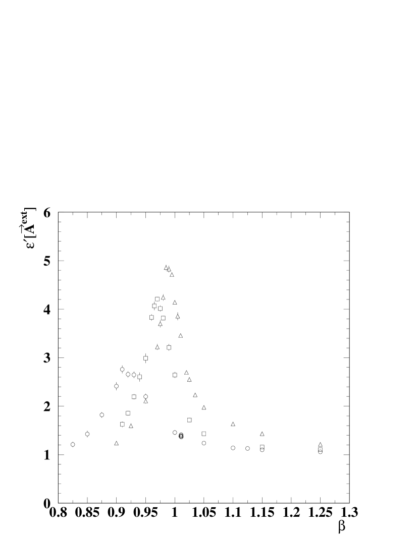
Figure 5: Figure 4 near the critical region $\beta\approx 1$.

References

- [1] U. Wolff, Nucl. Phys. B265 (1986) 506; ibid. 537.
- [2] M. Lüscher, R. Narayanan, P. Weisz, and U. Wolff, Nucl. Phys. B384 (1992) 168.
- [3] T. Banks, R. Myerson, and J. Kogut, Nucl. Phys. B129 (1977) 493.
- [4] T. A. DeGrand and D. Toussaint, Phys. Rev. D22 (1980) 2478.
- [5] W. Kerler, C. Rebbi, and A. Weber, Phys. Lett. B348 (1995) 560.
- [6] L. Del Debbio, A. Di Giacomo, and G. Paffuti, Phys. Lett. B349 (1995) 513; Nucl. Phys. B (Proc. Suppl.) 42 (1995) 231.
- [7] A. Hasenfratz, P. Hasenfratz, and F. Niedermayer, Nucl. Phys. B329 (1990) 739.
- [8] N. Barber, in Phase Transitions and Critical Phenomena Vol.8, C. Domb and J. E. Lebowitz eds., Academic Press, 1989.