M.C.R.G. Study of Fixed-connectivity Surfaces

Abstract

We apply Monte Carlo Renormalization group to the crumpling transition in random surface models of fixed connectivity. This transition is notoriously difficult to treat numerically. We employ here a Fourier accelerated Langevin algorithm in conjunction with a novel blocking procedure in momentum space which has proven extremely successful in $\lambda\phi^{4}$. We perform two successive renormalizations in lattices with up to $64^{2}$ sites. We obtain a result for the critical exponent $\nu$ in general agreement with previous estimates and similar error bars, but with much less computational effort. We also measure with great accuracy $\eta$. As a by-product we are able to determine the fractal dimension $d_{H}$ of random surfaces at the crumpling transition.

1 Introduction

The idea of implementing Wilson renormalization group [1] in numerical simulations was advocated by Swendsen in [2], where it was successfully applied to Ising spins. In this paper we shall use this approach to study the crumpling transition for fixed-triangulation surfaces.

In [3] it was proposed to add to the usual area or Nambu-Goto term [4] a piece proportional to the extrinsic curvature. The model has then a nontrivial $\beta$ function, the coupling being asymptotically free. An auxiliary metric can be introduced and the model interpreted as corresponding to $2d$ gravity coupled to interacting scalar fields. If one does not integrate over the auxiliary $2d$ metric the model admits a direct lattice transcription in terms of surfaces with fixed connectivity; i.e. crystalline surfaces[5], [6]. It is remarkable that for some intermediate value of the coupling $\kappa$ the model shows a second order phase transition. This transition will be the object of our interest.

Whenever one simulates a statistical system near a critical point one immediately faces the problem of critical slowing down. Critical slowing down is a consequence of the fact that near criticality the low momentum evolve very slowly with local algorithms. An algorithm that partially beats slowing down was introduced in [7] and uses a Fourier accelerated Langevin algorithm (FALA). This algorithm permits different updatings for different modes hence partially beating critical slowing down. FALA also facilitates a direct implementation of MCRG in momentum space by performing Kadanoff transformations that consist in decimations of the higher momenta, close to the original Wilson spirit[1]. A very successful application of these ideas to $\lambda\phi^{4}_{3}$ was presented in [8].

The organization of this paper is as follows. In section 2 we will give a general overview of the formal points of the method. In section 3 we will make a detailed discussion about the algorithm and the problems that need be circumvented in its applications. In section 4 we survey the previous work concerning the crumpling transition and fix some conventions. In section 5 we analyze extensively the results from our simulation and give estimates for the critical exponents. In section 6 we will point out some conclusions and possible extensions of this work.

2 The Method

The method we will use has been applied successfully to scalar theories[8]. Preliminary results dealing with the problem of surfaces have already appeared in[9]. In this section we will give a quick overview. Our starting point is a bare action

$$S=\sum_{\alpha}\lambda^{b}_{\alpha}O_{\alpha}^{b}$$ (1)

After applying a renormalization group transformation with a scale $t$ we end up with a similar action, but with renormalized couplings [1]: $\lambda_{\alpha}^{r}=F\left(\lambda_{\alpha}^{b}\right)$. We can linearize $F$ in the vicinity of the fixed point

$$\lambda_{\alpha}^{r}-\lambda_{\alpha}^{*}=\sum_{\beta}T_{\alpha\beta}\left(\lambda_{\beta}^{b}-\lambda_{\beta}^{*}\right),$$

$$T_{\alpha\beta}={\left(\frac{\partial\lambda_{\alpha}^{r}}{\partial\lambda_{\beta}^{b}}\right)}_{\lambda^{b}=\lambda^{*}}.$$ (2)

The largest eigenvalue $\lambda_{h}$ of $T_{\alpha\beta}$ will give the critical exponent $\nu$ according to the formula $\nu=\log t/\log\lambda_{h}$. Using the chain rule we get

$$\frac{\partial\langle O_{\lambda}^{r}\rangle}{\partial\lambda_{\beta}^{b}}=\sum_{\alpha}{\left(\frac{\partial\lambda_{\alpha}^{r}}{\partial\lambda_{\beta}^{b}}\right)\frac{\partial\langle O_{\lambda}^{r}\rangle}{\partial\lambda_{\alpha}^{r}}},$$ (3)

with

$$\frac{\partial\langle O_{\gamma}^{r}\rangle}{\partial\lambda_{\beta}^{b}}={\langle O_{\gamma}^{r}O_{\beta}^{b}\rangle}-{\langle O_{\gamma}^{r}\rangle\langle O_{\beta}^{b}\rangle},\qquad\frac{\partial\langle O_{\gamma}^{r}\rangle}{\partial\lambda_{\beta}^{r}}=\langle O_{\gamma}^{r}O_{\beta}^{r}\rangle-\langle O_{\gamma}^{r}\rangle\langle O_{\beta}^{r}\rangle.$$ (4)

These correlators and, in turn, $T_{\alpha\beta}$ and $\nu$ can be numerically computed.

A renormalization group transformation consists of a Kadanoff transformation that eliminates short distance degrees of freedom, and a rescaling of the fields. The Kadanoff transformation is largely arbitrary. The one we will use here will be a decimation in momentum space. At each step we will simply discard the high $p$ modes, half of them in each direction. This transformation can be implemented with a null cost in computer time and it has many advantages, as it will be evident in what follows. The rescaling of the fields is required in order that the normalization of a given operator (for example, the kinetic term in a scalar field theory) is preserved after each transformation. That amounts to redefining[1, 8]

$$\phi^{r}=\zeta\phi^{b}\quad\quad\quad\zeta=1/2^{(d+2-\eta)/2}$$ (5)

The quantity $\eta$ is, if computed at the fixed point, the conformal dimension of the field. In the case of surfaces is directly related to the Hausdorff dimension (see section 4). $\eta$ will be obtained selfconsistently by demanding that bare and renormalized observables should coincide at the fixed point. This delivers very precise values for $\eta$. Once $\nu$ and $\eta$ are determined we can get the rest of them through hyperscaling relations (see section 4).

It remains to select an efficient algorithm to compute the correlators (4). The crumpling transition has extremely long autocorrelation times near the critical point. autocorrelation times are surprisingly long (up to $10^{6}$ local updates in a $128\times 128$ system!) and that the asymptotic behaviour for the specific heat does not set in until the size of the system is relatively large. There is a whole industry of algorithms to overcome the problem of critical slowing down[12]. For the problem at hand, the crumpling transition, FALA[7] has been successfully employed[13, 14, 15, 9]. Its advantages are twofold: we partially beat critical slowing down and we can implement our Kadanoff transformation easily.

The implementation of the algorithm is not completely straightforward, however. It is thus worth to pause for one second and briefly digress on its foundations. We begin by constructing a random walk in configuration space via the stochastic Langevin equation

$$\phi(x,t_{n+1})=\phi(x,t_{n})+\Delta\phi(x,t_{n}),$$ (6)

$$\Delta\phi(x,t_{n})=-\Delta t\sum_{y}\epsilon(x,y)\frac{\partial S}{\partial\phi(y,t_{n})}+\sqrt{\Delta t}\ \eta(x,t_{n}),$$ (7)

where $\eta(x,t)$ is a gaussian noise which satisfies

$${\langle\eta(x,t)\eta(y,t^{\prime})\rangle}_{\eta}=2\delta_{t,t^{\prime}}\epsilon(x,y).$$ (8)

The choice $\epsilon(x,y)=\delta_{x,y}$ corresponds to a local updating which is more or less equivalent to the familiar Metropolis algorithm, with a dynamical exponent $z=2$. It has been used in random surfaces in [10], but suffers from long autocorrelation times and the same difficulties that will be discussed in the next section.

If we instead make the choice

$$\epsilon(x,y)=\sum_{p}\exp(-ip(x-y))\epsilon(p)$$ (9)

with a wise election of $\epsilon(p)$ we can accelerate separately the different Fourier modes. The equations after a simple rescaling read

$$\phi(p,t_{n+1})=\phi(p,t_{n})-\Delta t\epsilon(p){\cal F}\frac{\partial S}{\partial\phi(y,t_{n})}+\sqrt{\Delta t\epsilon(p)}\eta(p,t_{n}),$$ (10)

$$\langle\eta(p_{1},t)\eta(p_{2},t^{\prime})\rangle=2\delta_{t,t^{\prime}}\delta_{p1,-p2},$$ (11)

where ${\cal F}$ denotes the Fourier transform. In the previous equations the modes are manifest; by choosing a function $\epsilon(p)$ which enhances the low $p$-modes critical slowing down can be reduced as the longer equilibration times that low $p$-modes need are roughly made up by correspondingly larger updates.

From the previous Langevin equation one can derive the Fokker-Planck equation

$$P(\phi,t_{n+1})-P(\phi,t_{n})=\sum_{n=1}^{n=\infty}\sum_{x_{1},..,x_{n}}\frac{\partial}{\partial\phi(x_{1})}\frac{\partial}{\partial\phi(x_{2})}..\frac{\partial}{\partial\phi(x_{n})}\left(\Delta_{x_{1},x_{2},..,x_{n}}P(\phi,t_{n})\right),$$ (12)

$$\Delta_{x_{1},x_{2},..,x_{n}}=\frac{(-1)^{n}}{n!}\langle\Delta\phi(x_{1},t_{n})\Delta\phi(x_{2},t_{n})...\Delta\phi(x_{n},t_{n})\rangle,$$ (13)

whose stationary solution is, in powers of $\Delta t$,

$$P(\phi)=\exp\left(-S(\phi)+\frac{\Delta t}{2}\sum_{x,y}\epsilon(x,y)\left(\frac{\partial^{2}S}{\partial\phi(x)\partial\phi(y)}-\frac{1}{2}\frac{\partial S}{\partial\phi(x)}\frac{\partial S}{\partial\phi(y)}\right)+{\cal O}((\Delta t)^{2})\right)$$ (14)

The finiteness of the Langevin step induces unavoidable corrections to the Boltzmann distribution. The Langevin algorithm is not an exact one. These effects can be reduced by applying a slightly more complicated Langevin equation which cancels the ${\cal O}(\Delta t)$ corrections and is exact up to ${\cal O}({\left(\Delta t\right)}^{2})$

$$\phi(x,t_{n+1})=\phi(x,t_{n})-\frac{\Delta t}{2}\sum_{y}\epsilon(x,y)\left(\frac{\partial S}{\partial\phi(y,t_{n})}+\frac{\partial S(\bar{\phi})}{\partial\phi(y,t_{n})}\right)+\sqrt{\Delta t}\eta(x,t_{n})$$ (15)

$$\bar{\phi}(x,t_{n})=\phi(x,t_{n})-\Delta t\sum_{y}\epsilon(x,y)\frac{\partial S}{\partial\phi(y,t_{n})}+\sqrt{\Delta t}\eta(x,t_{n})$$ (16)

But in practice there is no real gain in doing so. A more interesting possibility is to make use of the hybrid algorithm[16]. This possibility in the context of random surfaces will be explored elsewhere.

To gain some insight on the size of the deviations of the equilibrium action with respect to the bare action one starts with it is useful to consider the effective action proposed in [13], which reproduces many features of the model. In this case we have a $p$-dependent renormalization of our parameters. For instance if $m$ is big enough the rigidity coupling changes as

$$\kappa\to\kappa(1+\frac{\pi^{2}\Delta t}{4}b)$$ (17)

where $b$ is a parameter which can be estimated and depends on $m$ and $\kappa$. We shall use Langevin steps in the region $\Delta t=10^{-5}$ to $\Delta t=10^{-4}$ and we conclude that the renormalization of the parameters due to the lack of exactness of the algorithm is of the order of $0.1\%$. We will see this explicitly when we obtain some observables.

3 The Praxis

In the previous section we described our method in very general terms. When the method confronts reality a number of technical issues have to be dealt with. We will set our simulation of crystalline random surfaces on a regular lattice with the topology of a torus. One of the advantages of FALA is the fact that the code is easily vectorized and parallelized. FALA involves the inversion of a matrix which with the help of fast Fourier transforms can be reduced to a manageable $N\log N$ computer cost, but only if our linear sizes are powers of 2.

When embedded in ${\bf R}^{3}$ each vertex has coordinates $x_{i}$ and each triangle has a normal $n_{I}$. The action contains two pieces: an ‘area’ term and a rigidity (extrinsic curvature) one. After scaling the surface tension to 1 it reads

$$S=\frac{1}{2}\sum_{i,j}{\left(x_{i}-x_{j}\right)}^{2}+\kappa\sum_{I,J}\left(1-n_{I}\cdot n_{J}\right)\equiv A+\kappa S_{EC}$$ (18)

(From now on we will stick to the following notation: sites and triangles are labelled with lowercase and uppercase indices, respectively). The partition function is

$$Z=\int\prod_{i}d^{3}x_{i}\delta^{(3)}(\sum_{i}x_{i})\exp{(-S)}$$ (19)

We must choose a precise form for $\epsilon(p)$ in (9). A physically motivated one would be

$$\epsilon(p)=\frac{\max_{p}\{\Delta\left(\Delta+m^{2}\right)\}}{\Delta\left(\Delta+m^{2}\right)},$$ (20)

where $m$ is the inverse correlation length $\xi$ and $\Delta$ is the lattice laplacian. The reason for this choice is that the above expression is —up to a constant— the exact two point function in the large $D$ limit[17], which is described by a gaussian theory. Gaussian models can be solved exactly by using a FALA and the optimum function $\epsilon(p)$ turns out to be the two point function. We shall use this form of $\epsilon(p)$ for $D=3$, but the optimal value for $m$ will turn out not to be $\xi^{-1}$.

The first point we have investigated is the need to incorporate a 2nd order algorithm as the one described in equations (15),(16). When compared to the simplest first order algorithm the computer time almost doubles. This additional time would not be a problem if one could make the Langevin step larger. As it is shown if fig. 1 the 2nd order algorithm gives a better approximation to the actual value, but to get acceptable results the Langevin step has to be of the same order of magnitude and no real gain in speed is obtained.

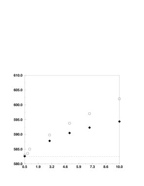
Figure 1: Comparison between first and second order Langevin algorithm. The expectation value of the curvature is plotted versus the Langevin step (in units of $10^{-4}$) for $N=256,\kappa=0.5$. The circles indicate the results obtained with a first order algorithm, filled diamonds with a second order one and the dashed lines are the exact result one would obtain with an exact algorithm (like Metropolis) by performing the simulation at the actual coupling.

Once this issue is settled, one notices immediately that the algorithm does not always reproduces the known results (some expectation values can be computed exactly, see section 5). The situation worsens for large Langevin steps and for large values of $\kappa$, but even for very small values of $\Delta t$ an analysis of the third dispersion of the area clearly shows abnormally large values. After dividing the data in small bins we can see the origin of the difficulties in fig. 2. From time to time a huge fluctuation takes place which spoils the statistical sample. Needless to say that a second order algorithm (or indeed any algorithm of any finite order) does not solve the problem. What is causing these fluctuations?

Figure 2: Average value of $A^{2}$ per bin as a function of the bin number. At bin number 22 there is a huge fluctuation.

It should be clearly understood that the huge fluctuations are an artifact of the algorithm requiring a finite $\Delta t$ and thus unphysical. To see this we can introduce a parameter $r$. At each step we measure the relative change of the observables; if it is greater than $r$, the whole configuration is rejected, we generate a new set of random numbers and go on. Typically one obtains that in $10^{5}$ configurations and $r=0.1$ just 5 or 6 configurations are rejected. With such small number of rejected configurations it is clear that the convergence to the Boltzmann configuration is not spoiled, but it is unclear whether all configurations that are rejected are truly ‘unphysical’. One also notices that while the number of such huge fluctuations is essentially independent of $\Delta t$, their magnitude does increase with the size of the Langevin step. The results are presented in Table 1.

$Observable$	$r=\infty$	$r=0.1$	$exact$
$A$	$387.7$	$381.1$	$382.5$
$\Delta A$	$758.1$	$406.7$	$382.5$
$\Delta^{2}A$	${\cal O}(10^{5})$	$927.3$	$765.5$
$S_{EC}$	$324.7$	$316.3$	$312.1$

Table 1: Results with and without rejection. $\Delta A$ and $\Delta^{2}A$ are the first and second dispersion of the area, respectively. The parameters of the run are: $N=16\times 16,\kappa=0.70$. No errors are shown.

If we examine the configuration immediately preceding the huge fluctuation we will see that it always contains a triangle of very small area. The derivative of the action in the extrinsic curvature term in the action in (18) has the form

$$n_{I}\cdot\frac{\partial n_{J}}{\partial x^{\alpha}_{k}}={1\over A_{J}}{\epsilon^{\beta\alpha\nu}\left(n_{I}^{\beta}-n_{I}\cdot n_{J}n_{J}^{\beta}\right){\left(x_{i}-x_{j}\right)}^{\nu}},$$ (21)

$I,J$ label neighbouring triangles, $i$,$j$,$k$ are the three vertices of triangle $J$. $A_{J}$ is the area of the triangle whose normal is $n_{J}$. If in eq.(21) $A_{J}$ is the area that shrinks to a small value the following update would blow up—except if $\Delta t$ is tiny, in which case thermalization would be problematic. In order to have a smooth integration of the Langevin equation the parameter which must be small at each step throughout the lattice is not $\Delta t$ but rather $\Delta t/A$. Now a smooth cut-off can be introduced according to this intuition [15]. Let us modify the extrinsic curvature term in (18) by

$$n_{I}\cdot n_{J}\rightarrow n_{I}\cdot n_{J}\exp\left(-s\Delta t\left({1\over A_{I}}+{1\over A_{J}}\right)\right),$$ (22)

where $s$ is a new dimensionless parameter. This change causes a negligible additional cost in time and formally does not spoil the convergence to the desired Boltzmann distribution as only the ${\cal O}(\Delta t)$ piece in (14) is affected. Of course since $\Delta t\neq 0$ in practice the observables are modified, although by fine tuning $s$ this modification can be made very small. Fine tuning the $s$ parameter is a real problem however as the optimal $s$ depends on $\Delta t$, $\kappa$, $m$ and even on the volume of the system. Tables 2, 3 show different values of $s$ and how they affect the observables for different choices of the parameters of the simulation. For the Langevin step that we will eventually use, $\Delta t=8\times 10^{-5}$ and for $m=1$ the optimal values for $s$ are: $s=10$ for $N=16\times 16$, $s=5$ for $N=32\times 32$ and $s=2$ for $N=64\times 64$, although small variations do not drastically alter the results. The introduction and ensuing fine tuning of $s$, although certainly a nuisance, are not expected to influence at all the critical behaviour on universality grounds; actually they may even provide for additional leeway in getting close to the fixed point.

$s$	$A$	$\Delta A$
$1$	$379.6$	$426.6$
$2$	$380.9$	$429.7$
$10$	$380.5$	$398.4$

Table 2: Dependence on $s$. Parameters of the run: $\kappa=0.80,N=16\times 16,m=1,N_{sweeps}=3\times 10^{5},\Delta t=6\times 10^{-5}$ The exact values are: $A=\Delta A=382.5$. No errors are shown.

$s$	$A$	$\Delta A$
$0.1$	$1542.1$	$1788.1$
$0.3$	$1539.8$	$1577.6$
$1$	$1539.2$	$1539.9$
$10$	$1538.4$	$1498.3$
$100$	$1536.2$	$1485.4$

Table 3: Dependence on $s$. Parameters of the run: $\kappa=0.80,N=32\times 32,m=1,N_{sweeps}=3\times 10^{5},\Delta t=8\times 10^{-5}$ The exact values are: $A=\Delta A=1534.5$. No errors are shown.

In principle we should expect that setting $m=1/\xi$ (the inverse of the correlation length) would lead to autocorrelation times growing logarithmically with the linear size of the system (that is $z=0$). Using $m=\xi^{-1}$ implies that near the critical surface very small values for $m$ have to be used. As it was observed in [13] the algorithm is then somewhat unstable and a larger value for $m$ had to be used in [13, 14, 15]. After extensive testing we decided to use $m=1$ in formula (20) in our FALA, We have also checked that larger values of $m$ do not bring any real improvement, provided that $\Delta t$ and $s$ are properly fine tuned. One should bear this in mind when comparing different Langevin simulations.

Let us now turn to the crucial issue of autocorrelation times. For a given observable (say the area) we consider

$$C_{A}(t)=\frac{\langle A_{t}A_{0}\rangle-\langle A_{t}\rangle\langle A_{0}\rangle}{\langle A_{0}^{2}\rangle-{\langle A_{0}\rangle}^{2}}.$$ (23)

For large values of $t$, $C_{A}(t)$ behaves as $C_{A}(t)=\exp(-t/\tau_{A})$, $\tau_{A}$ being the autocorrelation time of the observable $A$. The autocorrelation of the area turns out to be roughly independent of the volume of the system, but all the other observables autocorrelation times are certainly volume-dependent. Of all the measured autocorrelation times the one of $x^{2}$ is systematically the longest. The first thing one should worry is the dependence of the autocorrelation time on $\Delta t$, $m$ and $s$. For fixed $m$, a relation of the form $\tau_{A}\sim{1/\Delta t}$ holds, while the dependence on $s$ is negligible. Larger values of $m$ correspond to larger autocorrelation times as expected from the form of eq.(7). Some feeling on all these dependences can be gathered from figures 3 and 4.

Figure 3: Autocorrelation times for $S_{EC}$ at $\kappa=0.80$, $s=10$, $m=1$ as a function of $(\Delta t)^{-1}$ in units of $10^{3}$ (triangles). The squares show the dependence on $s$ of the autocorrelation time for $\Delta t=6\times 10^{-5}$, $\kappa=0.80$ and $m=1$, and correspond (left to right) to $s=1$, 2, 5 and 10. The diamonds show the dependence on $s$ of the autocorrelation time for $\Delta t=8\times 10^{-5}$, $\kappa=0.80$ and $m=0.125$, and correspond (left to right) to $s=1$, 10, 15, 20. In all cases the size is $16^{2}$ and the statistics $5\times 10^{5}$ sweeps.

Figure 4: Autocorrelation times for $x^{2}$ as a function of $\kappa$ for different volume sizes: circles $16\times 16$, filled diamonds $32\times 32$, squares $64\times 64$. In the latter case error bars are big due to the lack of enough statistics

In the light of the previous discussion it is clear that the most relevant decision is to choose a sound value for $\Delta t$. The best value is obtained by balancing systematic and statistical errors. $\Delta t$ must be small enough so that the equilibrium action is close enough to the bare action. Yet $\Delta t$ has to be large enough so that we get reasonably short autocorrelation times and thus manage to sample configuration space efficiently. The systematic error will be $\sigma_{syst}=a\Delta t$, where $a$ is a constant whose magnitude we can determine from the effective action proposed in [13] (see section 2) or simply estimate from our data. On the other hand, the statistical error will approximately be $\sigma_{stat}=\sqrt{\tau/N}$, $\tau$ being a typical autocorrelation time and $N$ the total number of sweeps that we can perform. We already know that $\tau=b(\Delta t)^{-1}$ (for fixed $\kappa$ the proportionality constant depends on $m$ and for $m=1$ is of ${\cal O}(10^{-2})$. Adding both errors in quadrature we get that the optimal $\Delta t$ is

$$\Delta t\sim(b/a^{2}N)^{1/3}$$ (24)

This yields Langevin steps of ${\cal O}(10^{-3})$. This argument is of course only indicative and further analysis shows that it is actually better to use a slightly smaller step, of ${\cal O}(10^{-4})$, the reason being that due to the difficulties that led to the introduction of the parameter $s$ the systematic errors are actually underestimated in the above argument.

4 The Crumpling Transition

The transition separating smooth from crumpled surfaces has attracted the attention of workers in string theory and condensed matter alike. There exist in the literature a variety of numerical and analytical studies. At this point is where the usefulness of a MCRG calculation becomes apparent. In the usual numerical studies only the exponent $\nu$ (and those related to it by hyperscaling relations) have been computed. In the analytical analysis only the exponents related to the Hausdorff dimension have been computed so far using a variety of approximations. MCRG gives first-principles estimates for both exponents in a single simulation.

Let us briefly review the definitions of the critical indices. The specific heat is defined as

$$C_{v}=\frac{\kappa^{2}}{N}\left(\langle S_{EC}^{2}\rangle-{\langle S_{EC}\rangle}^{2}\right).$$ (25)

In the scaling region, where the correlation length $\xi$ is large the exponents $\alpha$ and $\nu$ are defined by

$$C_{v}\sim{\left(\kappa_{c}-\kappa\right)}^{-\alpha},\qquad\xi\sim{\left(\kappa_{c}-\kappa\right)}^{-\nu}.$$ (26)

In [15] the well known hyperscaling relation $\alpha=2-\nu d$ has been tested numerically (within errors).

The Hausdorff or fractal dimension is defined by

$$\langle x^{2}\rangle\sim N^{2/d_{H}}.$$ (27)

It is related to the $x$-field anomalous dimension $\eta$ [10],[11] defined by

$$\langle x(\xi_{1})x(\xi_{2})\rangle\sim\frac{1}{{\|\xi_{1}-\xi_{2}\|}^{\eta}},$$ (28)

by the relation valid near $\kappa_{c}$

$$d_{H}=-4/\eta.$$ (29)

(Notice that this definition of $\eta$ is not the one used in [10].) We remark that $\eta$ must be a negative quantity, but from now on we will omit the negative sign in $\eta$.

It is common in models of $2d$ gravity to define a mass gap as the decay of the puncture-puncture correlation function. As the mass gap vanishes a critical index $\nu_{string}$ is defined. This $\nu_{string}$ is not related to $\nu$, but rather to the Hausdorff dimension $d_{H}$ by $d_{H}=1/\nu_{string}$.

The first numerical studies [5, 10] established the order of the transition. In [10] some estimates for the Hausdorff dimension were presented. They reported $d_{H}=4.0\pm 0.4$, although error bars were probably underestimated. In [5] the tentative estimate $d_{H}\simeq 3$ was presented but errors were not assessed. Many authors have obtained estimates for the critical exponents $\nu$ and $\alpha$. We summarize them in Table 4. We regard the results in [15] as the most reliable ones because they were obtained with bigger lattices and show a reasonable agreement between finite size analysis and a direct fit in the scaling region, while previous simulations [13],[14] and [21] were not entirely consistent. Obviously there is a lot of room for improvement in determining these exponents which should identify the relevant CFT at the transition.

Authors	$\alpha$	$\nu$	$\alpha(finitesize)$
[19]		$0.78(3)$	$0.44(5)$
[21]	$0.24(15)$	$0.89(8)$	$0.70(50)$
[20]		$0.60(20)$	$0.71(5)$
[15]	$0.58(10)$	$0.71(5)$	$0.54(10)$
[18]			$0.5$

Table 4: Current estimates of the critical indices associated to the crumpling transition

The first analytical studies were focused on the large $D$ properties [17], $D$ being the dimensionality of the ambient space. At $D=\infty$ the $\beta$ function can be computed exactly and there are no other zeroes than the trivial ones. In [11] a model very similar to the one we are considering was studied. The $\beta$ function was computed in the large $D$ limit including the first subleading term. Another fixed point was found and the Hausdorff dimension obtained, with the result[11] $d_{H}=2D/(D-1)$. At $D=3$, $d_{H}=3$. In [23] an $\epsilon$ expansion was performed for a variety of surface models. The relevant result for us is $d_{H}=2.73$, which is compatible with the previous one up to ${1/D}$ corrections. We are not aware of any analytical estimates for $\nu$.

5 The Results

In our renormalization group analysis we have considered 9 different operators. They are lattice transcriptions of simplified versions of the continuum operators that would appear in a derivative expansion. Their actual form is given in the Appendix. There is a large freedom in choosing the precise discretized form of a continuum operator, but the ambiguities associated to this freedom should correspond to irrelevant operators, representing non-universal corrections which vanish as positive powers of the lattice spacing modulo logarithms when the continuum limit is approached. Provided that the ones we include form a reasonably complete set with all the right symmetries up to a given dimension we should be on safe ground. We shall, at any rate, evaluate the errors associated to the truncation of the series of operators and to discretization ambiguities.

After elimination of the higher $p$-modes we Fourier transform back to position space and end up with a lattice with half the number of points in each direction. The rescaling factor discussed in section 2 will be determined by demanding that near a fixed point the expectation value of any bare and renormalized operators should coincide. We therefore allow $\eta$ to vary freely and choose the value that best fits this requirement. Only if we are close enough to the fixed point the rescaling of the fields has a universal meaning and is the conformal anomalous dimension. Some operators (those constructed with normals alone) contain no $x$-fields and therefore their matching will tell us in a unambiguous way how close we are to a fixed point. We have found that one blocking is not enough to bring us near the fixed point when we start with our bare original action, no matter how close to the critical surface we position ourselves. A second blocking is required to take us to the vicinity of the fixed point. Then the results are very satisfactory.

Let us consider the rescaling $x\rightarrow\lambda x$ in the bare action (18). Using this rescaling we can derive the following relations

$$\langle A\rangle=\frac{(N-1)D}{2},\qquad\langle A^{2}\rangle-{\langle A\rangle}^{2}=\frac{(N-1)D}{2},$$ (30)

$$\langle A^{3}\rangle-3\langle A^{2}\rangle{\langle A\rangle}^{2}+2{\langle A\rangle}^{3}=(N-1)D.$$ (31)

More relations, involving higher powers of $A$ may be obtained along the same lines, but they are of no use to us. These relations assume that the surface tension is set to unity, but it can be easily restored by dimensional analysis. To derive formulae (30) and (31) we have only assumed that the extrinsic curvature part of the action is scale invariant. If by any chance, after a renormalization group transformation, only operators involving normals are generated the above formulae should hold exactly. There is really no reason why higher dimensional operators containing powers of $x$ should not appear, but we can have an idea whether they trigger violations of the above scaling relations by checking the validity of (30),(31) after a renormalization group blocking.

At volume $32\times 32$ and $\kappa=0.82$ our simulation gives per site

$$\langle A\rangle=1.503\qquad\langle A^{2}\rangle=2.260\qquad\langle A^{3}\rangle=3.400$$ (32)

These results agree with those obtained from (30) and (31) after a tiny rescaling of $\mu$ (of ${\cal O}(10^{-3})$), showing that the surface tension does not get a large modification due to the use of the (non-exact) Langevin algorithm, in accordance with our expectations discussed in section 2. After blocking down to $16\times 16$ and choosing $\eta$ such that the same value of the area per site is reproduced we have

$$\langle A\rangle=1.503\qquad\langle A^{2}\rangle=2.260\qquad\langle A^{3}\rangle=3.404$$ (33)

The agreement, which is not peculiar to this value of $\kappa$ or to this volume, is impressive and it suggests that the effect of scale non-invariant operators is not very important.

We shall order the operators in the $T$ matrix in the following way: (a) operators made out of normals only, (b) operators that contain both normals and coordinates $x_{i}$ and (c) those which contain no normals at all. Within each group we shall order them by their dimensionality under the rescaling $x\to\lambda x$.

As we will see below the operators

$$\Delta x\Delta x,\qquad(\nabla x)^{4}$$ (34)

induce imaginary parts in the largest eigenvalue when they are included in the renormalization group analysis. We do not understand this fact very well. There is no reason to forbid these operators in our basis. In fact it was found in [13] that the large distance properties of crystalline random surfaces were well described by a term like the first one in eq. (34). This operator is nothing but another representation of the same operator as the extrinsic curvature itself (in fact some early simulations used this operator instead of $S_{EC}$ to represent the rigidity term). These operators are very sensitive to the actual value of $\eta^{*}$ one uses and by choosing a smaller value for the anomalous dimension the eigenvalues can be made real, but with large fluctuations. The second eigenvalue is then always very close to one. Of course the anomalous dimension must be gotten from the matching so this procedure is not consistent and must be discarded. (Incidentally, it is worth pointing out that the matching for these operators is as good as for the rest). We are inclined to believe that the difficulties with the imaginary parts could be solved by performing further blockings, as something similar happens with other operators when we compare the first and second blockings.

Our strategy has been the following. After finding the optimal values of $\Delta t$, $m$ and $s$, we run with the action (18) for different values of $\kappa$ until we get close to the critical surface from both sides (smooth and crumpled phases). Then we perform the following blockings: $64\times 64\to 32\times 32\to 16\times 16$, $32\times 32\to 16\times 16\to 8\times 8$ and $16\times 16\to 8\times 8$. We determine whether we are in the vicinity of the fixed point and if so proceed to measure $\nu$ and $\eta$. Additional runs have been used to measure the autocorrelations.

Preliminary results of our work were presented in [9]. Since then we have accumulated many more configurations and performed a second iteration of our renormalization group transformation, which has proven essential to pin down $\nu$ and, particularly, $\eta$. The results differ to some extent from those presented in [9] for reasons that will be explained below.

Error bars have three different origins. The statistical error is evaluated it by the usual binning procedures. We have good control over the autocorrelation times. In the case of a $64\times 64$ system the largest one (corresponding to $\langle x^{2}\rangle$) is in the range, $2000\sim 4000$ sweeps, fortunately by no means out of the reach of our computer facilities. The second source of errors are more difficult to assess. They have to do with the truncation of the number of operators entering the renormalization, the precise determination of the fixed point and, of course, $\Delta t$, errors as well as the uncertainties related to the $s$ parameter. And, last but not least, we have to deal with finite size errors. Critical exponents are affected by errors due to the influence of the finiteness of the lattice on the expectation values from which they are derived. However, what we call systematic errors (i.e. the dispersion in eigenvalues or errors due to truncation and discretization) are somewhat entangled with genuine finite size errors. This probably means that our error bars are probably overestimated.

All the numerical work was done with a CRAY-YMP, and SGI Power Challenge L. A first renormalization $32\times 32\rightarrow 16\times 16$ with 500,000 configurations takes about 1.5 hours of CPU time on a Cray-YMP. Applying twice the renormalization group to a $64\times 64$ system with a similar number of configurations in a SGI Power challenge L where three processors were fully used by our code takes about 52 hours of total CPU time or about 18 hours in real time.

5.1 First Renormalization

We shall not discuss in any detail the results of the $16\times 16\to 8\times 8$ blocking. It is only important to remark that many of the general trends are already present in such a small system. The value obtained for the anomalous dimension is $\eta=1.05(40)$. All errors quoted in this subsection merely reflect the systematic uncertainties due to the dispersion in values in the different operators and do not include statistical errors. The errors due to finite-size effects are not estimated here either. This is sufficient for our purposes.

Let us apply the MCRG to a system of size $32\times 32$ to get a $16\times 16$ lattice. We will present results for $\kappa=0.805$ (crumpled phase) and $\kappa=0.82$ (smooth phase) with $2\times 10^{6}$ sweeps each, although we have run for $\kappa$ values between 0.79 and 0.83. For $\kappa=0.805$ a correlation length of about 10 lattice units was reported to us [22], so finite size effects, though certainly present, are small. Unfortunately the blocking $32\times 32\to 16\times 16$ does not bring us close enough to the fixed point. (Recall that in $\lambda\phi^{4}_{3}$ one MCRG iteration was enough to get an excellent matching; obviously for rigid surfaces the fixed point lies far away from the canonical surface.) This is evidenced by the results presented in Tables 5, 6, where we estimate the anomalous dimension by attempting to match the bare and renormalized operators. Each operator requires a different $\eta$, with a large dispersion for the values, a clear signal that we are not yet in the vicinity of the fixed point, where an universal $\eta$ would suffice. Notice that the matching is not good for the operators $O_{1}$ to $O_{4}$ either, which depend only on normals and thus are $\eta$ independent.

	$32\times 32$	$16\times 16(\eta)$	$16\times 16$
$A$	$1.502$	$1.502(1.097)$	$1.462$
$A^{2}$	$2.259$	$2.260(1.097)$	$2.141$
$A^{3}$	$3.397$	$3.404(1.097)$	$3.139$
$S_{EC}^{2}$	$1.720$	$1.400$	$1.400$
$O_{1}$	$1.310$	$1.176$	$1.176$
$O_{2}$	$1.373$	$1.210$	$1.210$
$O_{3}$	$5.714$	$8.100$	$8.100$
$O_{4}$	$0.885$	$0.760$	$0.760$
$O_{5}$	$2.024$	$2.020(1.510)$	$2.617$
$O_{6}$	$1.998$	$2.040(1.55)$	$2.712$
$O_{7}$	$4.871$	$4.84(0.97)$	$3.725$
$O_{8}$	$4.465$	$4.33(0.7)$	$3.210$

Table 5: Matching between big and small lattices for $\kappa=0.805,s=5,m=1$. If we allow $\eta$ to vary independently for each operator and impose matching we obtain the values in the second column (the corresponding $\eta$ is shown in brackets). If instead we use the average $\eta$, which we call $\eta^{*}$, we obtain the values in the third column. The expectation values of the operators in this and in similar tables are given per site.

	$32\times 32$	$16\times 16(\eta)$	$16\times 16$
$A$	$1.503$	$1.502(1.124)$	$1.475$
$A^{2}$	$2.260$	$2.260(1.124)$	$2.180$
$A^{3}$	$3.400$	$3.404(1.124)$	$3.225$
$S_{EC}^{2}$	$1.597$	$1.256$	$1.256$
$O_{1}$	$1.262$	$1.113$	$1.113$
$O_{2}$	$1.295$	$1.114$	$1.114$
$O_{3}$	$5.404$	$7.420$	$7.420$
$O_{4}$	$0.848$	$0.711$	$0.711$
$O_{5}$	$1.997$	$2.000(1.524)$	$2.591$
$O_{6}$	$2.006$	$2.04(1.60)$	$2.782$
$O_{7}$	$4.864$	$4.88(0.96)$	$3.762$
$O_{8}$	$4.374$	$4.5(0.6)$	$3.104$

Table 6: Same as in the previous table, but for $\kappa=0.820$

In order to obtain $\nu$ and before proceeding to a second iteration of the renormalization group transformation we need to rescale the fields $x$ by choosing some prescription. The natural one is to demand that after a renormalization group transformation the normalization of the area term in the action is preserved. The fact that violations to the relations (30) and (31) are extremely small after a blocking suggests that, with very good accuracy, the blocked action has still the same invariance $x\to\lambda x$, $\mu\to\lambda^{-2}\mu$ that the original action had. Assuming that this symmetry is exact the absolute normalization of the area term in the blocked action can be obtained by comparing $\langle A\rangle$ and, say, $\langle A^{2}\rangle$, and the rescaling of the $x$-fields computed. If we were at the fixed point this rescaling would suffice to match all operators and would give to us the universal anomalous dimension $\eta$. When this is not quite the case, as it happens here, we simply use the rescaling obtained from the area and move on to the next blocking until we get close enough to a fixed point where a universal value for $\eta$ exists. Because in practice all observables are affected by errors it seems a good idea to use, to a limited extent, the rescalings which are suggested by operators other than the area too. We adopt a compromise solution were the final value of the rescaling that is used to derive $\nu$ is determined by performing a weighted average of the different values of $\nu$ in which area-type operators weigh more. Then we obtain $\eta^{*}=1.14(5)$ and $\eta^{*}=1.15(5)$ for $\kappa=0.805$ and $\kappa=0.820$, respectively. The $\chi^{2}/$d.o.f. is in both cases of ${\cal O}(100)$, which just reflects we are not quite at the fixed point. Using the values for $\eta^{*}$ obtained in this way we can determine the eigenvalues of the matrix $T$ and find $\nu=1.25(50)$. In short, $\eta^{*}$ cannot be interpreted as the anomalous dimension; it is just a convenient way of parametrizing the rescaling of the fields.

In the preliminary results presented in [9] only one blocking was being performed and the rescaling of the area was used to define the anomalous dimension. Although this is certainly a proper way of getting the rescaling of the fields, the resulting $\eta^{*}$ cannot be identified with the anomalous dimension because we were too far from the fixed point. We did, in fact, misjudged the distance to the fixed point. The second blocking results clarify this issue completely.

$\#$	$\kappa=0.805$	$\kappa=0.820$
$1$	$1.60$	$1.58$
$2$	$1.54$	$1.53$
$3$	$1.86$	$1.86$
$4$	$2.04$	$2.24$
$5$	$1.99$	$2.17$
$6$	$1.80$	$1.98$
$7$	$2.47*$	$2.59*$
$8$	$2.46*$	$2.59*$

Table 7: First blocking in the $32\times 32\to 16\times 16\to 8\times 8$ sequence. Evolution of the largest eigenvalue of the matrix $T$ as more and more operators are included in the MCRG. The asterisk indicates that the eigenvalue develops an imaginary part.

We can also apply one iteration of the MCRG to a system of $64\times 64$ down to $32\times 32$. For this size, autocorrelation for observables are relatively large (see fig. 4) and better statistics are required. Some $10^{7}$ configurations have been accumulated. We just present here the results for $\kappa=0.82$: $\eta^{*}=1.22(30)$, $\nu=1.06(30)$, with a $\chi^{2}/$d.o.f$\sim 10^{2}$. There is no real gain in precision and the results are not better than with smaller lattices. It is interesting to note that the ‘anomalous dimension’ increases with the volume.

5.2 Second Renormalization

From the results just discussed we conclude that the canonical surface is far from the fixed point. A second iteration of the renormalization group transformation should get us much closer. Closer in any case to the renormalized trajectory; that is, the trajectory that goes in the direction of the relevant operator of the theory near this fixed point. (We will later see that there is only one relevant direction.)

We shall apply the by now familiar machinery to the two-step blockings $32\times 32\to 16\times 16\to 8\times 8$ and $64\times 64\to 32\times 32\to 16\times 16$. Both the determination of $\eta^{*}$ and $\nu$ in the second iteration are independent of the value of $\eta^{*}$ used in the first one, although the precise numerical values of the different observables is sensitive to the first rescaling. In order to present our data we will take as the anomalous dimension of the first renormalization the one obtained from equations (30),(31) for the reasons discussed in the previous subsection. After following the usual strategy we see in Tables 8, 9 the results of the second blocking. It is obvious that there is a tremendous improving with respect to the results presented in Tables 5, 6. We no longer have a large dispersion in the $\eta$ exponent and the matching is now much better. For operators that are made only of normals the agreement is at the $20\%$ level. Relations such as (30),(31) are satisfied with very good accuracy.

If we perform a least square fit (now with equal weights for all operators) we get for $\kappa=0.805$ $\eta^{*}=1.41(20)$ while at $\kappa=0.820$ we get $\eta^{*}=1.44(20)$. In both cases $\chi^{2}/$d.o.f$\simeq 50$. The Hausdorff dimension is $d_{H}=2.83(23)$. In spite of the still somewhat big error bars we can already compare with the analytical estimates of section 4 with good agreement.

	$16\times 16$	$8\times 8(\eta)$	$8\times 8$
$A$	$1.502$	$1.500(1.400)$	$1.491$
$A^{2}$	$2.260$	$2.261(1.400)$	$2.231$
$A^{3}$	$3.400$	$3.415(1.400)$	$3.365$
$S_{EC}^{2}$	$1.400$	$2.350$	$2.350$
$O_{1}$	$1.176$	$1.522$	$1.522$
$O_{2}$	$1.210$	$1.177$	$1.177$
$O_{3}$	$8.101$	$12.44$	$12.44$
$O_{4}$	$0.760$	$1.000$	$1.000$
$O_{5}$	$2.689$	$2.690(1.490)$	$2.750$
$O_{6}$	$2.750$	$2.700(1.34)$	$2.534$
$O_{7}$	$3.931$	$3.931(1.378)$	$3.720$
$O_{8}$	$3.300$	$3.34(1.6)$	$3.730$

Table 8: Matching between big and small lattices after the second iteration of the MCRG on a $32\times 32$ system. $\kappa=0.805,s=5,m=1$

	$16\times 16$	$8\times 8(\eta)$	$8\times 8$
$A$	$1.502$	$1.500(1.433)$	$1.491$
$A^{2}$	$2.260$	$2.260(1.433)$	$2.231$
$A^{3}$	$3.404$	$3.420(1.433)$	$3.365$
$S_{EC}^{2}$	$1.260$	$2.174$	$2.174$
$O_{1}$	$1.113$	$1.459$	$1.459$
$O_{2}$	$1.115$	$1.670$	$1.670$
$O_{3}$	$7.420$	$11.73$	$11.73$
$O_{4}$	$0.713$	$0.960$	$0.960$
$O_{5}$	$2.640$	$2.635(1.50)$	$2.750$
$O_{6}$	$2.833$	$2.800(1.30)$	$2.534$
$O_{7}$	$3.900$	$3.901(1.405)$	$3.720$
$O_{8}$	$3.161$	$3.3(1.6)$	$3.730$

Table 9: Matching between big and small lattices after the second iteration of the MCRG on a $32\times 32$ system. $\kappa=0.820,s=5,m=1$

Let us now compare the values of$\langle x^{2}\rangle$ in the big and small lattices

$$\langle x^{2}\rangle_{16\times 16}=4.84,\qquad\langle x^{2}\rangle_{8\times 8}=1.78.$$ (35)

Using (see previous section)

$$d_{H}=\frac{4\log 2}{\log{\langle x^{2}\rangle_{N}}-\log{\langle x^{2}\rangle_{\frac{N}{2^{d}}}}}$$ (36)

we obtain $d_{H}=2.77(10)$ in good agreement with the one already obtained. We can even check the consistency by employing higher cumulants of $x^{2}$ and still obtain the same result.

With the above values for $\eta^{*}$ we get the series of eigenvalues displayed in Table 10. The eigenvalues are all bigger than 2, implying a second order transition. We obtain $\nu=0.87(10)$. Error bars just reflect the dispersion of the eigenvalues of the $T$ matrix; no statistical or finite-size errors are considered yet.

$\#$	$\kappa=0.805$	$\kappa=0.820$
$1$	$2.08$	$2.04$
$2$	$2.10$	$2.05$
$3$	$2.34$	$2.24$
$4$	$2.30$	$2.21$
$5$	$2.32$	$2.36$
$6$	$2.28$	$2.33$
$7$	$1.99*$	$2.09*$
$8$	$1.91*$	$2.00*$

Table 10: Second blocking in the $32\times 32\to 16\times 16\to 8\times 8$ sequence. Evolution of the largest eigenvalue of the matrix $T$ as an increasing number of operators are included in the MCRG.

The above results are very encouraging, but not fully satisfactory yet. It is clear that the matching is much better, implying that we are in the vicinity of the fixed point. Perhaps it should not be surprising that the dispersion in $\eta$ is still large because after the second application of the MCRG to a $32\times 32$ lattice we end up with a $8\times 8$ lattice. In principle we should not have any more difficulties on a $8\times 8$ lattice than we had in the original $32\times 32$ one since at the same time that the lattice is reduced the correlation length is reduced by exactly the same amount. We try to keep severe finite size effects under control by running at values of $\kappa$ which are close enough to the critical surface, yet with a correlation length smaller than our system size. However the ‘critical’ behaviour for such small lattices shows a rather erratic pattern[21] with the critical region being significantly shifted. In spite of this the results are reasonably good, showing that the method is very robust.

It is clear that larger systems are called for. Let us now turn to the $64\times 64\rightarrow 32\times 32\to 16\times 16$ sequence of blockings. While several values of $\kappa$ were investigated in smaller lattices, due to computer time availability here we will run only at $\kappa=0.805$ and $\kappa=0.82$, collecting up to $10^{7}$ configurations. The enlargement of the lattice size brings about a little miracle. We see at once from Tables 11, 12 that the matching between bare and renormalized operators is now wonderful, particularly for $\kappa=0.820$. The dispersion in the anomalous dimension reduces now to a narrow width. Note that operators that are insensitive to the anomalous dimension show agreement which is in some cases as good as a $1\%$. This is a matching of the same quality as the one obtained in [8] and it is the one we were after.

	$32\times 32$	$16\times 16(\eta)$	$16\times 16$
$A$	$1.496$	$1.496(1.55)$	$1.545$
$A^{2}$	$2.238$	$2.237(1.55)$	$2.401$
$A^{3}$	$3.349$	$3.3525(1.55)$	$3.705$
$S_{EC}^{2}$	$0.695$	$0.740$	$0.740$
$O_{1}$	$0.830$	$0.852$	$0.852$
$O_{2}$	$0.694$	$0.760$	$0.760$
$O_{3}$	$4.431$	$4.902$	$4.902$
$O_{4}$	$0.508$	$0.510$	$0.510$
$O_{5}$	$2.451$	$2.453(1.51)$	$2.467$
$O_{6}$	$3.002$	$3.010(1.53)$	$3.065$
$O_{7}$	$3.763$	$3.752(1.50)$	$3.741$
$O_{8}$	$2.556$	$2.51(1.45)$	$2.42$

Table 11: Matching between big and small lattices after the second iteration of the MCRG on a $64\times 64$ system. $\kappa=0.805,s=2,m=1$

	$32\times 32$	$16\times 16(\eta)$	$16\times 16$
$A$	$1.503$	$1.503(1.585)$	$1.565$
$A^{2}$	$2.260$	$2.260(1.585)$	$2.451$
$A^{3}$	$3.397$	$3.400(1.585)$	$3.843$
$S_{EC}^{2}$	$0.555$	$0.553$	$0.553$
$O_{1}$	$0.744$	$0.740$	$0.740$
$O_{2}$	$0.573$	$0.606$	$0.606$
$O_{3}$	$3.617$	$3.889$	$3.889$
$O_{4}$	$0.448$	$0.435$	$0.435$
$O_{5}$	$2.382$	$2.382(1.525)$	$2.380$
$O_{6}$	$3.039$	$3.034(1.567)$	$3.120$
$O_{7}$	$3.757$	$3.760(1.527)$	$3.768$
$O_{8}$	$2.387$	$2.36(1.45)$	$2.200$

Table 12: Matching between big and small lattices after the second iteration of the MCRG on a $64\times 64$ system. $\kappa=0.820,s=2,m=1$. The statistical error is $\pm 0.002$ in all observables.

We notice that for $\kappa=0.82$ we are particularly close to the fixed point after two iterations, although $\kappa=0.805$ is also good. We will draw our conclusions from the former value of $\kappa$ were matching is slightly better. The results are then

$$\eta^{*}=1.527\pm 0.010\pm 0.006\pm 0.020$$ (37)

with a $\chi^{2}/$d.o.f$\simeq 1$. Errors due to truncation, statistics and finite size effects are separately quoted (in this order; see the discussion at the beginning of this section). We remind the reader that to obtain the true anomalous dimension of the field one should reverse the sign of $\eta^{*}$. The Hausdorff dimension is

$$d_{H}=2.62\pm 0.02\pm 0.01\pm 0.04$$ (38)

Where the first error comes from the dispersion of the anomalous dimensions, the second one is statistical and the third one an estimate of the error due to finite size effects. A self consistent computation of $d_{H}$ along the lines of equation (36), considering that from our simulation we get,

$$\langle x^{2}\rangle_{32\times 32}=20.98(8),\qquad\langle x^{2}\rangle_{16\times 16}=7.33(13),$$ (39)

yields

$$d_{H}=2.64(5),$$ (40)

in good agreement with the previous estimate. Only the statistical error is included.

A look at the table of eigenvalues shows that the dispersion has reduced tremendously when compared to the previous cases. From the results in Table 13

$$\nu=0.85\pm 0.07\pm 0.02\pm 0.06$$ (41)

The first error bar corresponds to the systematic uncertainty of the method, the second one corresponds to statistical errors, and the third one estimates finite size errors, as before. Adding all errors in quadrature we get $\nu=0.85\pm 0.09$.

$\#$	$\lambda_{h}$
$1$	$2.25(-)(2)$
$2$	$2.23(-)(2)$
$3$	$2.22(-)(2)$
$4$	$2.15(-)(3)$
$5$	$2.20(3)(5)$
$6$	$2.18(3)(5)$
$7$	$2.19(6)(6)*$
$8$	$2.18(6)(6)*$

Table 13: Second blocking in the $64\times 64\to 32\times 32\to 16\times 16$ chain. Evolution of the largest eigenvalue of the matrix $T$ as a function of the number of operators included in the MCRG. The first error is due to the uncertainty in the anomalous dimension $\eta^{*}$ (it does not affect ops. 1-4), while the second one reflects the statistical error.

In the $T$ matrix all the other eigenvalues are smaller than one so there is only one relevant direction in the theory. We can give a tentative value for the first subleading exponent $\omega$,

$$\omega=-0.35^{+0.25}_{-0.50}.$$ (42)

Equations (37) to (42) are our final results. If we compare our results with previous determinations (see section 4) we see that they are in reasonable agreement. $\nu$ is slightly higher than the most recent estimates, with similar error bars. $d_{H}$ is slightly lower than the theoretical predictions. The amount of numerical work required to determine $\nu$ is however substantially smaller than with other methods and, of course, we can determine $d_{H}$ directly with a good assessment of the errors involved and, perhaps more importantly, we gain a very good understanding of the crumpling transition. For instance, it is very interesting to see how the renormalization group brings together after two blockings the trajectories that started at both sides of the critical surface.

5.3 $\beta$ Function

MCRG has permitted us to compute the critical exponents but we have said very little about the flow of the renormalization group and the effective action one obtains after integrating high $p$-modes. Within our framework it is not possible to compute the renormalized couplings so these important problems would require a separated study. However, something can be said about the general form of the $\beta$ function. There are two realistic scenarios as shown in figure [5]. Our results give strong support that case B is the one that is realized, even if the evidence is not fully conclusive.

Let us consider the quantity $R_{rg}$, defined as

$$R_{rg}=\frac{\langle S_{EC}\rangle_{N}}{2^{d}\langle S_{EC}\rangle_{\frac{N}{2^{d}}}},$$ (43)

That is $R_{rg}$ is the ratio of the average of extrinsic curvatures before and after renormalization with the convenient factor that makes it an intensive quantity. Now, if $R_{rg}>1$ then the surface is less crumpled in the infrared whereas if $R_{rg}<1$ it becomes more crumpled as we move to larger distances. On a $64\times 64$ lattice at $\kappa=0.83$ we can compute the average extrinsic curvature and obtain

$$\langle S_{EC}\rangle_{64\times 64}=4829(2),\qquad\langle S_{EC}\rangle_{32\times 32}=857(1).$$ (44)

Then at $\kappa=0.83$ (smooth phase) we have $R_{rg}=1.50$, clearly the surface is less crumpled in the infrared, in agreement with case B.

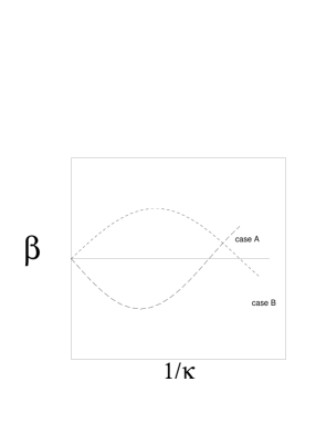
Figure 5: $\beta$ as a function of $1/\kappa$ in arbitrary units. The two relevant cases for us are depicted, In case A the origin is an ultraviolet fixed point while in case B it is infrared stable.

We can see this behaviour in another way. We apply MCRG at $\kappa=0.83$ and we end up with a smaller lattice. Let us make an estimate of the value of $\kappa_{eff}$ which we would have to use in the small system to obtain the value quoted in (44). A look at a simulation in a system $32\times 32$[19] shows that $\kappa_{eff}>0.9$ so the flow goes according to case B. The analysis for other $\kappa$ values is also as clean in giving evidence for the same shape of the $\beta$-function.

Unfortunately in the crumpled phase things are not so clear. If we work with a system at $\kappa=0.79$ we obtain that $R_{rg}=1.05(10)$ and at $\kappa=0.81$ $R_{rg}=1.12(10)$. $R_{rg}$ seems to be greater than one, but only marginally so, as the case $R_{rg}<1$ cannot be excluded within error bars. On the other hand a look at the second renormalization gives at $\kappa=0.79$, $R_{rg}=0.8$, now the ratio indeed becoming smaller than 1. In the crumpled phase we have no conclusive evidence on the flow of the $\beta$ function.

6 Conclusions

The crumpling transition separating rigid and crumpled surfaces has been object of intense scrutiny over the last decade. In this paper we have presented a fresh approach to the problem of determining the critical exponents associated to that critical point. We have analyzed the transition using Monte Carlo renormalization group techniques combining a Fourier accelerated Langevin algorithm with a thinning of degrees of freedom directly in momentum space. Where comparison is possible we have found good agreement with the most recent simulations and found with great accuracy the value of the fractal dimension at the critical point. We have also given clear evidence of the existence of a fixed point towards which all trajectories in the vicinity of the critical surface are driven as well as the existence of a unique relevant direction. We can confidently claim that our results are well established and have passed all the necessary validity tests to be trusted.

More computer resources should allow a thorough investigation of a system of size $128\times 128$ where it should be possible to perform three successive blockings. In the light of the present experience as well as the one gained from $\lambda\phi^{4}$ we believe that such a simulation would deliver the exponent $\nu$ with a 1% precision (our level of precision here on $\nu$ is at the 10% level). The precision on $\eta$ could easily reach the per mille level (our current precision on $\eta$ is 2%). Such a work would give very clear evidence about the nature of the transition and with little additional effort it would be possible to follow the renormalization group trajectories. It would certainly shed some light on some technical difficulties we encountered such as the problems associated to the operators (34). The interesting thing is that given the autocorrelation times obtained using FALA such system is by no means out of reach of existing computer facilities. However, to remove some systematic uncertainties that we have encountered the use of a hybrid algorithm in combination with blocking in momentum space would be preferable.

Since the nature of the transition in three dimensions it is by now well understood, an important question that remains open is the nature of the transition in higher dimensions. In the first studies of such models [5],[10] it was clearly established that the transition gets weaker as the dimension is increased, but nothing could be said about the order of the transition for $D>4$ or the existence of an upper critical dimension above which there is no transition at all. To settle down these issues more work has to be done and certainly MCRG will be a decisive instrument.

Another point of great interest would be to implement such renormalization group calculations to the case where we switch on gravity[24]. The latest numerical simulations with such systems[25] suggest that the transition becomes then of third order. Numerical simulation are extremely time consuming for such models, and, up to know, there are no reliable estimates for the critical exponents. It seems plausible that a combination of $2d$ gravity renormalization group methods, like the ones using self-similarity of the triangulations[26] and the one described in this paper could shed some light on this very important issue. Alternatively, Regge calculus with a non-local action taking proper care of the conformal anomaly can also be attacked by the same techniques. Work on this latter approach is now under way.

Acknowledgements

We would like to thank J. Wheater for discussions, correspondence and for sharing some of his results with us. Discussions with D.Johnston are also gratefully acknowledged. We would like to thank Ll. Garrido for expert advice on computing issues, and CESCA and CEPBA for making their machines available to us. A.T. acknowledges a grant from the Generalitat de Catalunya. This work has been supported in part by UE contract CHRX-CT93-0343 and CICYT grant AEN93-0695.

Appendix A Appendix

In the continuum we classify operators according to their canonical dimensions $d_{c}$. Recalling that $x$ is a dimensionless field in two dimensions, a possible exhaustive list would be

$d_{c}=2$: $\nabla x\nabla x$.

$d_{c}=0$: $Tr{K^{2}}$ and $R$.

$d_{c}=-2$: $Tr{K^{4}}$, $Tr{K^{3}}Tr{K}$, $(Tr{K^{2}})^{2}$, $Tr{\nabla K\nabla K}$, $(Tr{\nabla K})^{2}$, $R\ TrK^{2}$ and $R^{2}$. In the above expressions $K$ is the second fundamental form of the surface and $R$ the gaussian curvature. We did not consider operators odd in $x$ such as $trK$ as they are not present in the bare action and will never be generated in the course of a renormalization group transformation. We do not include in our analysis any operator containing $R$ as we think that the transition is driven by terms feeling the ambient space only.

Figure 6: Conventions used in the discretizations of the operators.

In order to discretize the above operators it is convenient to introduce the following conventions. Given a site $i$, $j(i)$ runs over the neighbouring sites. The same convention applies to triangles, $J(I)$ runs over the triangles adjacent to triangle $I$. Given a site $i$ and a nearest neighbour $j(i)$ which selects a direction in our triangular lattice with sixfold symmetry, we name the neighbouring triangles in the manner depicted in fig. 6

$$TrK=\sum_{j(i)}\left(n_{I}-n_{K_{1}}\right)\cdot\left(x_{j}-x_{i}\right)$$ (45)

$$TrK^{2}=\frac{1}{2}\sum_{J(I)}{\left(n_{I}-n_{J}\right)}^{2}=\sum_{J(I)}(1-n_{I}\cdot n_{J})$$ (46)

$$TrK^{3}=\sum_{j(i)}\left(n_{I}^{\mu}n_{K_{1}}^{\nu}\right)\left(x^{\nu}_{j}-x^{\nu}_{i}\right)\left(n_{K_{2}}^{\mu}+n_{K_{3}}^{\mu}\right)$$ (47)

$$TrK^{4}=\sum_{J(I)}(1-n_{I}\cdot n_{J})^{2}$$ (48)

$$(Tr\nabla K)^{2}=\sum_{j(i)}{\left(\frac{1}{3}\left(n_{K_{3}}+n_{K_{4}}\right)\cdot\left(x_{i}-x_{j}\right)\right)}^{2}$$ (49)

$$Tr\nabla K\nabla K=\Delta n_{I}\cdot\Delta n_{I}$$ (50)

where the laplacian acting on $x$’s and $n$’s are defined by

$$\Delta x_{i}=\sum_{j(i)}{\left(x_{i}-x_{j}\right)}$$ (51)

$$\Delta n_{I}=\left(n_{I}-\frac{1}{3}\sum_{J(I)}n_{J}\right)$$ (52)

These are the building blocks of our discretization. It is important to ensure that symmetries of the bare action like parity or discrete rotational symmetry are preserved by the terms that we considered. To ensure the latter we have symmetrized our operators when necessary. The naming conventions of the different operators as appear in the body of the paper are displayed in Table 14.

$O_{1}$	$TrK^{2}$
$O_{2}$	$Tr(K^{2})^{2}$
$O_{3}$	$(TrK^{2})^{2}$
$O_{4}$	$Tr(\nabla_{a}K\nabla_{a}K)$
$O_{5}$	$TrKTrK^{3}$
$O_{6}$	$(Tr\nabla K)^{2}$
$O_{7}$	${\left((\nabla_{a}x)^{2}\right)}^{2}$
$O_{8}$	$\Delta x\Delta x$

Table 14: List of operators.

While the discretization of some operators (in particular those involving only normals) is rather natural, this is not so in other cases. To get a feeling of the errors involved in the discretization procedure we have also tried the following ones

$$TrK=\sum_{j(i)}{\left(n_{K_{1}}-n_{K_{2}}\right)\cdot\left(x_{i}-x_{j}\right)}$$ (53)

$$TrK^{3}=\left(\sum_{j}\left(x_{i}^{\mu}-x_{j}^{\mu}\right)\left(n_{K_{1}}^{\nu}-n_{K_{2}}^{\nu}\right)\right)\left(\sum_{j}\left(n_{K_{1}}^{\mu}-n_{K_{2}}^{\mu}\right)\left(n_{K_{1}}^{\nu}-n_{K_{2}}^{\nu}\right)\right)$$ (54)

We have changed accordingly $O_{5}$ and $O_{6}$.

The results show only very slight modifications. For instance after including the new discretizations we get a similar pattern of eigenvalues with no significative improvement except perhaps that some of the imaginary parts become actually smaller with the new discretization and the dispersion of eigenvalues is slightly reduced. For instance in a $32\times 32\to 16\times 16\to 8\times 8$ blocking at $\kappa=0.82$ we got with $6\times 10^{5}$ configurations the sequence of eigenvalues: 2.08, 2.07, 2.21, 2.19, 2.18, 2.19, 1.96, 1.92, whose average is 2.10. (to be compared with the average 2.17 in Table 10).

References

- [1] K.Wilson and J. Kogut, Phys. Rep. 12 (1974), 75
- [2] R.H. Swendsen, Phys. Rev. Lett. 42 (1979), 859
- [3] W. Helfrich J. Phys. 46 (1985) 1263 A. Polyakov Nucl. Phys. B268 (1986), 859 H. Kleinert Phys. Lett. 174B (1986), 335
- [4] Y. Nambu, Copenhagen symposium on strings, 1970, unpublished T. Goto Prog. Theor. Phys. 46(1971) 1560
- [5] M.Baig, D.Espriu and J.Wheater, Nucl. Phys. B314 (1989), 587.
- [6] Y. Kantor and D. Nelson Phys. Rev. Lett. 58 (1987), 2774
- [7] G.G. Batrouni, G.R. Katz, A.S. Kronfeld, G.P. Lepage, B. Svetitsky and K.G. Wilson, Phys. Rev. D32 (1985), 2736.
- [8] D.Espriu and A. Travesset, Phys. Lett. 356B (1995), 329
- [9] D.Espriu and A. Travesset, hep-lat/9509062, to appear in Nucl. Phys. B (Proc. Supp.)
- [10] J. Ambjorn, B. Durhuus and T. Jonsson, Nucl. Phys. B316 (1989), 526.
- [11] F. David and E. Guiter, Europhys. Lett. 5 (8) 709 (1988)
- [12] A.D. Sokal, Nucl. Phys. B(Proc. Supp.) 20 (1991), 247.
- [13] R. Harnish and J. Wheater, Nucl. Phys. B350 (1991), 861.
- [14] J. Wheater and P. Stephenson, Phys. Lett. 302B (1993), 447.
- [15] J.Wheater, Oxford preprint OUTP-95-07-P, to be published in Nucl. Phys. B
- [16] S. Duane, A.D. Kennedy, B.J. Pendleton and D. Roweth, Phys. Lett. 195B (1985), 216 A. Horowitz Phys. Lett. 268B (1991), 247 A.L. Ferreira and R. Toral Phys. Rev. E47 (1993) 3848
- [17] F. Alonso and D.Espriu , Nucl. Phys. B283 (1987), 393; F. David and E.Gutter , Nucl. Phys. B295 (1988), 332; K. Kirsten and V.F. Muller, Zeitsch. f. Physik C45 (1989), 159.
- [18] K. Anagnostopoulos et al., hep-lat 9509074, to appear in Nucl. Phys. B (Proc. Supp.)
- [19] R. Renken and J. Kogut, Nucl. Phys. B342 (1990), 753
- [20] B. Petersson and B. Jegerlehner, Nucl. Phys. B(Proc. Supp.)34 (1994), 723
- [21] M.Baig, D.Espriu and A. Travesset, Nucl. Phys. B426 (1994), 575.
- [22] J. Wheater ,private communication
- [23] P. Le Doussal and L. Radzihovsky, Phys. Rev. Lett. 69 (1992), 1209
- [24] S. Catterall, Phys. Lett. 220B (1989), 207 C. Baillie, D. Johnston and R. Williams Nucl. Phys. B335 (1990), 469 C. Baillie, D. Johnston and R. Williams Nucl. Phys. B354 (1991), 295 J. Ambjorn et al., Phys. Lett. 275B (1992), 295
- [25] J. Ambjorn et al., Nucl. Phys. B393 (1993), 571 M. Bowick et al., Nucl. Phys. B394 (1993), 791 K. Anagnostopoulos et al. Phys. Lett. 317B (1993), 102
- [26] D. Johnston, J.P. Kownacki and A. Krzywicki Nucl. Phys. B(Proc. Supp.)42 (1995), 728 Z. Burda, J.P. Kownacki and A. Krzywicki Phys. Lett. 356B (1995), 466 S. Catterall and G. Thorleifsson hep-lat 9510003