DFTUZ 96/1

A multisite microcanonical updating method

Abstract

We have made a study of several update algorithms using the XY model. We find that sequential local overrelaxation is not ergodic at the scale of typical Monte Carlo simulation time. We have introduced a new multisite microcanonical update method, which yields results compatible with those of random overrelaxation and the microcanonical demon algorithm, which are very much slower, all being incompatible with the sequential overrelaxation results.

Microcanonical local algorithms are used often in numerical simulations of spin systems or lattice gauge theories. Sometimes they are used in combination with canonical algorithms in order to accelerate decorrelation in Monte Carlo time. Some other times one is interested in a pure microcanonical simulation for physical reasons [1, 2, 3]. We do not consider nonlocal microcanonical methods which are based on molecular dynamics and are used specially for studying dynamical fermions[4].

Possibly, the most popular microcanonical algorithm is Local Microcanonical Overrelaxation (LMO) [5]. The algorithm, simple and fast, has a dynamical exponent $z=1$ when the update is done sequentially, and $z=2$ when it is done randomly [6], the difference being due to a wave effect occurring in the former case, which causes the change made in the update of a variable to propagate to the next one, the updated configuration being farther from the original one than in the case consecutive updates had been made independently. Yet, no proof exists of the algorithm being ergodic. Its determinism, particularly in the case of sequential update, might induce one to think that it is not ergodic. Indeed, we shall present evidence of the lack of ergodicity of the sequential LMO method.

We shall introduce here the Multisite Microcanonical method (MM), a new microcanonical updating algorithm which exchanges energy among different regions of the lattice at each update. It has two features which are absent from the LMO: it is non-local and non-deterministic. They contribute to diminishing Monte Carlo correlation time, and avoid the biases that plague LMO.

Apart from the mentioned LMO and MM, we have also done simulations using the Microcanonical Demon Algorithm, (MDA), introduced by Creutz [7], in order to have one further point of reference.

We have chosen a simple model for our simulations, the two dimensional XY model. We remark that the method could be easily generalized to O($N$) models in arbitrary dimensions, or even to abelian and SU(2) gauge theories.

In what follows, we shall recall the two dimensional XY model, introducing the observables we have measured, and study the mentioned algorithms, LMO, MDA and MM.

In a square lattice of side $L$, with periodic boundary conditions, we define on each site a variable $\phi(n)\in U(1)$, the action

$$S=\sum_{n,\mu}{\rm Re\hskip 5.69054pt}\phi(n)\phi^{*}(n+\mu)$$ (1)

and the density of states with energy E

$$N(E)={\cal Z}^{-1}\int\prod_{n}d\phi(n)\delta(S(\phi)-E).$$ (2)

${\cal Z}$ being the partition function.

The presented results have been obtained in a $64^{2}$ lattice, with a normalized energy value $E=0.4453$, which corresponds to $\beta\sim 1.0$. The data plotted in figures have been obtained with $45,000$ configurations (after thermalization). Where the results were not conclusive we have added $500,000$ MC iterations. Most runs have been started from two fixed (thermalized) configurations. Errors have been calculated using the jackknife method.

Among the measured observables, the energy, the process being microcanonical, should remain constant. We have measured it as a check of the different methods, observing small changes due to rounding errors in the microcanonical methods, and larger oscillations in the MDA case, because in the latter only the total energy (system plus demon) remains constant.

We have measured the total magnetization, defined as $M=\frac{1}{L^{2}}\sum_{n}\phi(n)$. $M$ being a complex number, we have measured its modulus and phase, which, although it can be chosen arbitrarily by a global gauge change, $\phi(n)\to U\phi(n)$, $\forall n,\ U\in{\rm U}(1)$, can give us a hint on how the system is evolving.

The most useful observables for our study have turned out to be the spatial correlations. In particular, we have measured the correlation between parallel lines at distances from $0$ to $L/2$, i.e., defining

$$\omega(x)=\frac{1}{L}\sum_{y}\phi(x,y)\qquad\omega(y)=\frac{1}{L}\sum_{x}\phi(x,y)$$ (3)

(where the notation $\phi(x,y)$ has been used, instead of $\phi(n)$), the correlation at a distance $r$ is written

$$\eta(r)=\frac{1}{2}\langle\omega(x)\omega^{*}(x+r)+\omega(y)\omega^{*}(y+r)\rangle.$$ (4)

We have studied separately the real and imaginary parts of $\eta(r)$. From the real part, correlation lengths can be extracted.

The imaginary part should be zero at any $r$, due to the symmetry of the action under the transformation $\phi(n)\to\phi^{*}(n),\forall n$. We shall see that the imaginary part is not zero in the LMO method. This implies that the system does not evolve uniformly in the whole phase-space, so breaking the fundamental assumption of the microcanonical ensemble: at any time, all the states of the system with the given energy have equal probability.

Let us consider first the LMO algorithm. Writing $\phi=e^{i\theta(n)}$ and defining

$$\rho(n_{0})e^{i\alpha(n_{0})}=\sum_{\pm\mu}e^{-i\theta(n_{o}+\mu)},$$ (5)

the action associated to the site $n_{0}$ reads

$$S(n_{0})={\rm Re\hskip 5.69054pt}(\phi(n_{0})\sum_{\pm\mu}\phi^{*}(n_{0}+\mu))=\rho(n_{0})\cos(\theta(n_{0})+\alpha(n_{0})).$$ (6)

One LMO step consists on picking a site $n_{0}$ and updating $\theta(n_{0})$ to a new value

$$\theta^{\prime}(n_{0})=-\theta(n_{0})-2\alpha(n_{0})$$ (7)

which, due to the parity of the $\cos$ function, does not alter the energy.

The step satisfies detailed balance in a deterministic way: the probability of going from one state to the other is $1$ in both senses. But a simulation takes many of these steps, and the order in which they are taken is also important. If we question the relationship between two states separated by $N$ such steps, taking the intermediate sites randomly satisfies detailed balance, but taking them sequentially does not. The looser condition of balance [6, 8] is satisfied, though. The latter, together with ergodicity, is sufficient for the algorithm to reproduce the desired distribution after a reasonable number of sweeps. However, the determinacy of each single step makes one question the ability of the method to satisfy ergodicity. Running a sweep forward and backwards would leave the configuration unchanged. Also, a sequential overrelaxation sweep on a one-dimensional XY model would have as only effect to transport a little energy packet along the chain, leaving the rest of the chain undisturbed.

Proving ergodicity is, in general, difficult, but disproving it may be easier. A proof of lack of ergodicity is the occurrence of results which, in the limit of infinite statistics, depend on the initial state. Also, finding a conserved quantity which should not be conserved means that the algorithm runs in a certain region of phase space, characterized by a certain value of the conserved quantity, without being able to leave it.

Figure 1: Evolution in Monte Carlo time of the phase of the magnetization for several algorithms. Only a sample of each run is shown.

Let us consider sequential LMO, SLMO. Fig. 1a shows that the phase runs over the interval $(-\pi,\pi]$ at a practically constant rate (we shall call that property helicity). The sign and modulus of the helicity depend on the initial configuration, and they are kept through the simulation with small fluctuations. We have consistently used two fixed configurations, characterized by their respective large and small value of the helicity, as initial configurations in all our simulations, in order to check the possible dependence of the results on the initial state. Making the necessary allowances for the proviso made above on the meaning of the phase, the origin of the rotation described being a global rotation of the system would be of no importance, but problems might arise if the rotations were local.

The imaginary part of the spatial correlation defined above, Im$(\eta(r))$, should average statistically to zero, the quantity being invariant under a global rotation, but sensitive to local ones. Fig. 2a shows that SLMO yields values for Im$(\eta(r))$ clearly incompatible with zero within the statistical errors, statistics being sufficiently high. That, together with the fact that other algorithms do yield results fully compatible with zero, confirms our suspicion that SLMO does not run over the phase space properly.

As Im$(\eta(r))$ is not either a very usual observable, we have considered too Re$(\eta(r))$. Fig. 3a shows that SLMO yields results incompatible with each other and dependent on the helicity of the initial configuration. In order to reinforce this conclusion we have increased the statistics with $500,000$ more iterations, with results confirming the incompatibility.

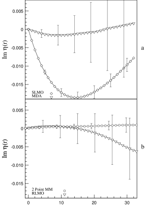
Figure 2: Imaginary part of the spatial correlation evaluated by several algorithms (with $50,000$ iterations in each case).

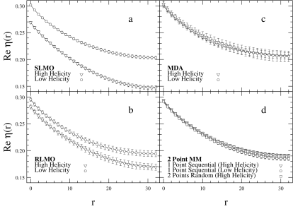
Figure 3: Real part of the spatial correlation evaluated by several algorithms (with $50,000$ iterations in each case).

Randomly ordered LMO (RLMO) does not conserve helicity. In that case, the phase of $M$, shown in Fig. 1b, evolves very slowly in a nonsystematic way. Fig. 2b shows that Im$(\eta(r))$ is compatible with zero. However, Fig. 3b shows that the real part is also dependent on the initial configuration, although the values are less different from each other than in the SLMO case, and the errors, also for $|M|$, are much bigger, and so are the correlation times. Clearly, it would be wrong to infer from the error size that SLMO is better than RLMO, as we know by now that the former runs only over a small region of phase space.

Next, we have run also up to $500,000$ iterations for each initial configuration (high and low helicity) and in this case the results for Re$(\eta(r))$ have changed dramatically with respect to those obtained with $50,000$ iterations. Now the results for the two different starts become fully compatible (and compatible also with those obtained by other methods shown later). Therefore RLMO behaves ergodically, but with a Monte Carlo time scale very large compared with the scale of the other algorithms shown later.

It must be said, in discharge of SLMO, that despite its lack of ergodicity, the fact that it decorrelates efficiently, in the sense that it produces configurations which, although all belong to a restricted region of phase space, are fairly far from each other, can, as has been widely shown, make it very useful when combined with other algorithms, like Metropolis, which reinstate ergodicity.

Let us consider next the Microcanonical Demon Algorithm, in which an extra degree of freedom, the demon, travels through the system, transferring energy from one point to another. The total energy of the system plus the demon is kept constant, which makes the algorithm to be not strictly microcanonical from the point of view of the system alone. The algorithm works as follows: a small amount of absolute energy is assigned initially to the demon, say, 1. When updating a spin, a new random tentative value is chosen, and the new system energy is computed. In case it increases, the change is accepted, and the excess energy is given to the demon. If the energy decreases, the change is accepted only if the demon energy is sufficient to provide the difference, the demon energy being always kept non-negative.

As only one demon is being used (more demons can be included in the formalism) and its initial energy is small, the system evolves in a practically microcanonical way. Fig. 1c shows the evolution of the phase of $M$, which shows no helicity. Fig. 2a shows Im$(\eta(r))$ calculated by the MDA. As can be seen, it is compatible with 0. In Fig. 3c we plot the results of the algorithm for Re$(\eta(r))$ for the two fixed initial configurations, showing the independence of the evolution from the initial state.

Next, we introduce our Multisite Microcanonical method, which is a non-local, non-deterministic algorithm allowing the exchange of energy among different sites, keeping the system energy constant.

Using the notation introduced in (5) we rewrite the system energy as

$$E=\frac{1}{2}{\rm Re}\sum_{n,\pm\mu}\phi(n)\phi^{*}(n+\mu)=\frac{1}{2}\sum_{n}\rho(n)\cos(\theta(n)+\alpha(n))\equiv\frac{1}{2}(\vec{\rho},\vec{x})\ .$$ (8)

Keeping a constant energy means keeping constant the scalar product of the two vectors $\vec{\rho}$ and $\vec{x}$ just defined:

$$(\vec{\rho},\vec{x})=K$$ (9)

The expression is valid for the energy of a subset of any $N$ sites, the vectors $\vec{\rho}$ and $\vec{x}$ being now $N$-dimensional. If, moreover, the set does not contain interacting sites, updating the set means changing the vector $\vec{x}$, as $\vec{\rho}$ and the $\alpha^{\prime}$s remain constant in the process.

The algorithm proceeds as follows: $N$ non-interacting sites are chosen, $\vec{\rho}$ and $\vec{x}$ are computed, a new $\vec{x}^{\prime}$ is generated in such a way that $(\vec{\rho},\vec{x}^{\prime})=(\vec{\rho},\vec{x})$ and the new variables $\theta^{\prime}$ are obtained from $\vec{x}^{\prime}$.

Yet, many technical details must be kept in mind. The components of the vector $\vec{x}^{\prime}$ being cosines, must lie in the interval $[-1,1]$, and, when computing the new values $\theta^{\prime}$, one has the freedom to choose the sign of $\sin(\theta^{\prime}+\alpha)$, maintaining detailed balance. One possibility is choosing it with equal probability for both signs, another is to include a measure of overrelaxation, choosing the sign which yields the $\theta^{\prime}$ which lies farther away from the original one.

But, in order to ensure ergodicity and balance, it is the $\phi^{\prime}$ space (or equivalently, the $\theta^{\prime}$ space) which must be filled uniformly. Once we have generated the $\vec{x}^{\prime}$s uniformly, we can get a uniform distribution in the $\theta^{\prime}$ space weighting the configurations with the Jacobian of the transformation from the $\theta^{\prime}$s to the $\vec{x}^{\prime}$s, which is

$$J(\theta\to x)=\prod_{n}\frac{1}{\sin(\theta(n)+\alpha(n))}$$ (10)

so that, once we have generated uniformly the new $\vec{x}^{\prime}$ we keep it or not with a probability proportional to the quotient of the new and old jacobians.

Our problem reduces, then, to uniformly generating points in a $(N-1)$-dimensional polyhedron, which is the intersection of the $N$-dimensional solid hypercube of side two centred in the origin and the $(N-1)$-dimensional hyperplane perpendicular to $\vec{\rho}$ containing $\vec{x}$.

An obvious way to generate $\vec{x}$ uniformly is generating uniformly $(N-1)$ components in the interval $[1,-1]$, and finding the $N$th component which ensures that $\vec{x}$ lies in the hyperplane. In case the last component lies in the interval $[1,-1]$, one accepts the new point, otherwise one must start and try again. Clearly, the inefficiency of this method grows exponentially with $N$, making the method useless for other than a few sites.

The largest set of non-interacting sites is the set of all equally coloured sites in the checkerboard lattice, which contains $N=V/2$ points, which for an interesting lattice is of the order of thousands, which makes the use of such inefficient methods hopeless.

We have explored other more sofisticated methods, on which we shall report elsewhere, but in general one must trade acceptance for computational load, the net result being the unimplementability of the method for large $N$. We have relaxed the demand to generate uniformly at each step, still insisting on keeping detailed balance, but then the explored region becomes small, and the decorrelation is poor.

Turning to MM with small $N$, $N=1$ is local and corresponds to LMO. $N=2$ is the smallest value which allows a non-local update, and consequently an energy exchange between arbitrarily different sites (LMO exchanges energy only between the ends of a link). That, together with the fact that at $N=2$ the efficiency of the method is highest, the geometrical acceptance rate being one, as will be shown later, has moved us to choose $N=2$.

Having chosen the value of $N$, the problem remains of how to pick the two non-interacting sites. The most unbiased choice is picking them at random (RMM), and that has been done. Yet, we have mentioned that sequential updating has the advantage of a wave effect, which transmits the decorrelation effect along the sequence, so we have basically done simulations moving one site sequentially and picking the other one at random, which seems to be efficient.

Figure 4: Intersection of the solid hypercube of side 2 centered in the origin with the hyperplane perpendicular to $\vec{\rho}$ containing $\vec{x}$ in two dimensions.

With $N=2$, the equation

$$\rho_{1}x_{1}+\rho_{2}x_{2}=K$$ (11)

must be satisfied, $x_{1}$ and $x_{2}$ being uniformly distributed in the allowed region. That is easily done; one looks for the maximum and minimum values of $x_{1}$ for which a solution for $x_{2}$ to (11) exists between $-1$ and $1$, and then a value for $x_{1}$ is generated randomly and uniformly in that interval. Fig. 4 illustrates the process.

Let us call $(x_{1},x_{2})$ the old values of $\vec{x}$ and $({x^{\prime}}_{1},{x^{\prime}}_{2})$ the new ones, generated as described above. From them the values of the new $({\theta^{\prime}}_{1},{\theta^{\prime}}_{2})$ are obtained, solving $x^{\prime}=\cos(\theta^{\prime}+\alpha)$. Next, in order to obtain uniformly distributed $\theta^{\prime}$s, the quotient $C$ of jacobians is computed

$$C=\frac{{(\sin({\theta^{\prime}}_{1}+{\alpha^{\prime}}_{1})\sin({\theta^{\prime}}_{2}+{\alpha^{\prime}}_{2}))}^{-1}}{{(\sin({\theta}_{1}+{\alpha}_{1})\sin({\theta}_{2}+{\alpha}_{2}))}^{-1}}$$ (12)

and the new values are accepted if $C\geq 1$, or otherwise with probability proportional to C. The acceptance from this factor becomes around 70%. Finally we have chosen to take the sign of $\sin(\theta^{\prime}+\alpha)$ which yields the farthest $\theta^{\prime}$ from the original one.

The results of the simulation with the implementation of the MM algorithm just described, are as follows: Fig. 1d shows the evolution of the magnetization phase, which rambles unsystematically. Fig. 2b shows that Im$(\eta(r))$ is compatible with $0$, with much smaller errors than for other algorithms. Fig. 3d , in which results of RMM runs are included, shows that Re$(\eta(r))$ behaves identically for both initial configurations and both implementations of the algorithm, with smaller errors for the choice sequential-random.

MM results for Re$(\eta(r))$ are just outside error bars with respect to MDA results. This is due to the fact, already mentioned, that MDA simulations are not strictly microcanonical, and in fact the energy values of the MDA simulation, which run in the range $(0.4550,0.4562)$, yield a slightly higher mean value than those of the MM simulations, which range in $(0.4552,0.4553)$ (due to rounding). This explains qualitatively why the MDA results are slightly bigger than the MM ones. This situation is unavoidable, if we insist on studying the dependence of the results on the initial state, which forces us to use fixed initial states for all our simulations, so losing in a certain measure our control on the average energy in the case of MDA.

Forgetting about helicity, we have run with MM at energy $0.4556$ (the mean energy of MDA) and in this case the results are compatible.

The comparison with the LMO results in Fig. 3a,b is pointless, since those results are selfincompatible.

Our conclusions are, then:

SLMO is not ergodic (for the two-dimensional XY model).

We have introduced a new multisite, microcanonical update method, MM.

Among the microcanonical algorithms studied here, SLMO and MM have proved to be the most efficient, as far as Monte Carlo time decorrelation is concerned, although LMO runs only over a restricted region of phase space.

The RLMO, MDA and MM algorithms yield compatible results, while LMO results are start-dependent and incompatible.

We wish to thank Juan J. Ruiz-Lorenzo for useful discussions. Partially supported by CICyT AEN93-0604-C03, AEN94-0218, AEN95-1284E, and ERBCHRXCT920051. D.I. is a MEC Fellow.

References

- [1] F. R. Brown, A. Yegylalp, Phys. Lett. 155A, 252 (1991).
- [2] P. Stolorz, Phys. Lett. 172B, 77 (1986).
- [3] V.Azcoiti et al, Phys. Rev. Lett. 65, 2239 (1990); Phys. Rev. D48, 402 (1993).
- [4] J. Polonyi and H.W. Wyld Phys. Rev. Lett. 51, 2257 (1983). D. Callaway and A. Rahman Phys. Rev. D28, 1506 (1983).
- [5] M. Creutz, Phys. Rev. D36, 515 (1987).
- [6] A. Sokal in ”Quantum fields in the Computer”, Advanced series of Directions in High Energy Physics, Vol 11, p.211, Editor M. Creutz, World Scientific (1992).
- [7] M. Creutz, Phys. Rev. Lett. 50, 1411 (1983).
- [8] G. Parisi, ”Statistical Field Theory”, Addison Wesley (1988).