Long range correlations in branched polymers.

Abstract

We study the correlation functions in the branched polymer model. Although there are no correlations in the grand canonical ensemble, when looking at the canonical ensemble we find negative long range power like correlations. We propose that a similar mechanism explains the shape of recently measured correlation functions in the elongated phase of 4d simplicial gravity[1].

1 Introduction

Recently some measurements of the curvature–curvature correlation functions in 4d simplicial gravity were presented [1]. The data seems to indicate negative and power like behavior both at the transition and in the elongated phase. The latter seems surprising as one would expect the exponential decay of correlations outside the critical region. Those issues are hard to study numerically and even harder analytically. To gain some insight into possible mechanism of those correlations we investigate here a simple geometrical model: branched polymers (BP).

Besides its simplicity there are some other motivations for using this model. The BP describe the $c\rightarrow\infty$ limit of 2d simplicial gravity [2, 3]. It is believed that BP also describe the elongated phase of 4d simplicial gravity [4]. However the exact correspondence between the quantities measured in ref. [1] and BP is not known. Nevertheless we can hope that the BP model captures the general features of the elongated phase of 4d simplicial gravity.

2 The model

We consider here the ensemble of planar rooted planted trees. A tree is a graph without the closed loops. A rooted tree is a tree with one marked vertex (root) and planted tree is a tree whose root’s degree (number of branches) is one. Two trees are considered as distinct if they cannot be mapped on each other by a continuous deformation of the plane (see fig. 1).

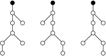
Figure 1: Example of distinct planted rooted trees

We denote by $n$ the total number of non-root vertices in the tree and by $n_{i}$ the number of non-root vertices of the degree $i$. Then the (grand) partition function is defined as

$$Z(\mu,t)=\sum_{T\in{\cal T}}e^{-\mu n}\rho(T),\qquad\rho(T)=t_{1}^{n_{1}}t_{2}^{n_{2}}\cdots$$ (1)

The ${\cal T}$ denotes the ensemble of all the trees. The equation for $Z(\mu,t)$ is (see fig. 2) [2]

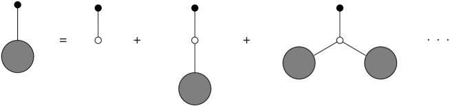
Figure 2: Partition function

$$Z(\mu,t)=e^{-\mu}{\cal F}(Z(\mu,t))\quad\text{with}\quad{\cal F}(Z)=\sum_{i=1}^{\infty}t_{i}Z^{i-1}.$$ (2)

The equation (2) can be rewritten as

$$e^{\mu}=\frac{{\cal F}(Z)}{Z}$$ (3)

and the critical point $\mu_{c}$ corresponds to a value $Z_{0}$ where the right hand side of (3) has a minimum. In the neighborhood of this point for a large class of parameters $t$ the partition function behaves like [2]

$$Z(\mu,t)\approx Z_{0}(t)-Z_{1}(t)\sqrt{\Delta\mu}+Z_{2}(t)\Delta\mu+O(\Delta\mu^{\frac{3}{2}})$$ (4)

with $\Delta\mu=\mu-\mu_{c}$. That is the only class of solutions of the equation (2) considered in this paper. Behaviour described by (4) is typical also for the elongated phase of the 4d simplicial gravity [4]. From the equation (2) we can derive

$$\begin{split}Z_{0}&=\frac{{\cal F}(Z_{0})}{{\cal F}^{(1)}(Z_{0})},\\ Z_{1}&=\sqrt{\frac{2{\cal F}(Z_{0})}{{\cal F}^{(2)}(Z_{0})}},\\ Z_{2}&=\frac{1}{3}\frac{{\cal F}(Z_{0})}{{\cal F}^{(2)}(Z_{0})^{2}}(3Z_{0}{\cal F}^{(2)}-{\cal F}^{(3)}(Z_{0})),\end{split}$$ (5)

where ${\cal F}^{(i)}=\frac{\partial^{i}{\cal F}}{\partial Z^{i}}$.

3 The Two-Point functions

First we consider a “volume–volume” correlation function [3]

$$G(\mu,t;r)=\sum_{T\in{\cal T}_{r}}e^{-\mu n}\rho(T)$$ (6)

where ${\cal T}_{r}$ is the ensemble of the trees with one point marked at distance $r+1$ from the root.

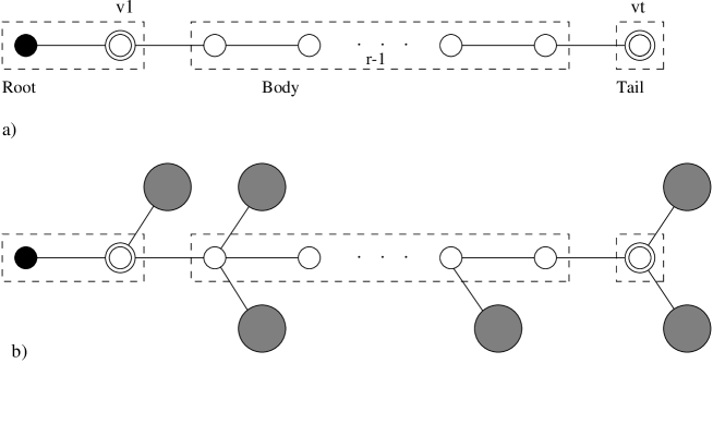
Figure 3: Two-point function

The smallest possible tree in ${\cal T}_{r}$ is a chain of $r+1$ non-root vertices which we split into root, body and tail (see fig. 3a). The weight of this chain is $t_{1}t_{2}^{r}e^{-(r+1)\mu}$. All other configurations in ${\cal T}_{r}$ can be obtained from this chain by attaching trees in its non-root vertices(see fig. 3b). Attaching $n$ trees in the body or root part of the chain corresponds to a factor $t_{n+2}(n+1)Z^{n}$. The factor $n+1$ counts the possible relative positions of the chain. Attaching $n$ trees to the tail corresponds to a factor $t_{n+1}Z^{n}$. Finally our two-point function is

$$\begin{split}G(\mu,t;r)=&e^{-\mu}(t_{2}+2t_{3}Z+3t_{4}Z^{2}+\cdots)\cdot\\ &\cdot e^{-(r-1)\mu}(t_{2}+2t_{3}Z+3t_{4}Z^{2}+\cdots)^{r-1}e^{-\mu}(t_{1}+t_{2}Z+\cdots)\\ =&e^{-\mu}{\cal F}^{\prime}(Z)e^{-(r-1)\mu}{\cal F}^{\prime}(Z)^{(r-1)}e^{-\mu}{\cal F}(Z)=(1+\frac{Z}{Z^{\prime}})^{r}Z\end{split}$$ (7)

where ${\cal F}^{\prime}(Z)=\frac{\partial{\cal F}(Z)}{\partial Z}$ and $Z^{\prime}=\frac{\partial Z(\mu,t)}{\partial\mu}$. In the last equality we used the identity $e^{-\mu}{\cal F}^{\prime}(Z)=1+\frac{Z}{Z^{\prime}}$ obtained by differentiating the equation (2) with respect to $\mu$.

We are interested in the Root-Tail correlation function defined as follows:

$$RT(\mu,t;r)=\sum_{{\cal T}_{r}}d(v_{1})d(v_{r+1})e^{-\mu n}\rho(T)$$ (8)

where $d(v)$ is the degree of vertex $v$. The form of this function can be easily obtained by modifying $G(\mu,t;r)$

$$\begin{split}RT(\mu,t;r)=&e^{-\mu}(2\cdot t_{2}+3\cdot 2t_{3}Z+4\cdot 3t_{4}Z^{2}+\cdots)\cdot\\ &\kern-28.45274pt\cdot e^{-(r-1)\mu}(t_{2}+2t_{3}Z+3t_{4}Z^{2}+\cdots)^{r-1}e^{-\mu}(1\cdot t_{1}+2\cdot t_{2}Z+\cdots)\\ =&e^{-\mu}\frac{1}{Z}\frac{\partial({\cal F}^{\prime}(Z)Z^{2})}{\partial Z}e^{-(r-1)\mu}{\cal F}^{\prime}(Z)^{(r-1)}e^{-\mu}\frac{\partial({\cal F}(Z)Z)}{\partial Z}\\ =&(2+\frac{4Z}{Z^{\prime}}+\frac{Z^{2}}{{Z^{\prime}}^{2}}-\frac{Z^{2}Z^{\prime\prime}}{{Z^{\prime}}^{3}})(1+\frac{Z}{Z^{\prime}})^{(r-1)}(2Z+\frac{Z^{2}}{Z^{\prime}})\end{split}$$ (9)

where we used the identity $e^{-\mu}F^{\prime\prime}(Z)=\frac{2}{Z^{\prime}}+\frac{Z}{{Z^{\prime}}^{2}}-\frac{ZZ^{\prime\prime}}{{Z^{\prime}}^{3}}$ again obtained by differentiating eq. (2) twice with respect to $\mu$.

Similarly we define two other functions

$$\begin{split}R(\mu,t;r)=&\sum_{T\in{\cal T}_{r}}d(v_{1})e^{-\mu n}\rho(T)=(2+\frac{4Z}{Z^{\prime}}+\frac{Z^{2}}{{Z^{\prime}}^{2}}-\frac{Z^{2}Z^{\prime\prime}}{{Z^{\prime}}^{3}})(1+\frac{Z}{Z^{\prime}})^{(r-1)}Z,\end{split}$$ (10)

$$\begin{split}T(\mu,t;r)=&\sum_{T\in{\cal T}_{r}}d(v_{r+1})e^{-\mu n}\rho(T)=(1+\frac{Z}{Z^{\prime}})^{r}(2Z+\frac{Z^{2}}{Z^{\prime}}).\end{split}$$ (11)

Let

$$\langle A\rangle_{{\cal T}_{r}}=\frac{\displaystyle\sum_{T\in{\cal T}_{r}}A(T)e^{-\mu n}\rho(T)}{\displaystyle\sum_{T\in{\cal T}_{r}}e^{-\mu n}\rho(T)}.$$ (12)

We define the normalized connected Root-Tail correlation function as

$$\begin{split}RT_{c}(\mu,t;r)&=\langle(d(v_{1})-\langle d(v_{1})\rangle_{{\cal T}_{r}})(d(v_{r+1})-\langle d(v_{r+1})\rangle_{{\cal T}_{r}})\rangle_{{\cal T}_{r}}\\ &=\frac{RT(\mu,t;r)}{G(\mu,t;r)}-\frac{R(\mu,t;r)T(\mu,t;r)}{G(\mu,t;r)^{2}}.\end{split}$$ (13)

It is easy to check that

$$RT_{c}(\mu,t;r)\equiv 0.$$ (14)

4 The canonical ensemble

The functions defined in the preceding chapter are the discrete Laplace transforms of their canonical counterparts e.g.

$$G(\mu,t;r)=\sum_{n=0}^{\infty}e^{-\mu n}G(n,t;r)\quad\text{with}\quad G(n,t;r)=\sum_{T\in{\cal T}_{r}(n)}\rho(T)$$ (15)

where ${\cal T}_{r}(n)$ is the ensemble of the trees belonging to ${\cal T}_{r}$ and having exactly $n$ non-root vertices. To calculate the canonical functions from grand canonical we have to perform the inverse of the discrete Laplace transform. This usually can not be done exactly and we proceed with a series of approximations.

The first approximation is that of replacing the discrete transform (15) with the continuous one. Then $G(n,t;r)$ is given by the inverse Laplace transform which we calculate by the saddle point method. The details are presented in appendix A. Below we give results to the leading order in $n$ ($r\ll n$).

$$\begin{split}G(n,t;r)\approx&\frac{1}{2\sqrt{\pi}}Z_{0}xn^{-\frac{3}{2}}\,e^{\mu_{c}n}\exp\left(-\frac{1}{4n}x^{2}\right),\end{split}$$ (16)

$$\begin{split}RT(n,t;r)\approx&\frac{2}{\sqrt{\pi}}Z_{0}\left(x\frac{Z_{0}^{2}+Z_{1}^{2}}{Z_{1}^{2}}-\frac{Z_{0}(Z_{0}^{2}+6Z_{0}Z_{2}-5Z_{1}^{2})}{Z_{1}^{3}}\right)n^{-\frac{3}{2}}\,e^{\mu_{c}n}\cdot\\ &\cdot\exp\left(-\frac{1}{4n}\left(x-\frac{Z_{0}}{Z_{1}}\frac{(Z_{0}^{2}+6Z_{0}Z_{2}-5Z_{1}^{2})}{Z_{0}^{2}+Z_{1}^{2}}\right)^{2}\right),\end{split}$$ (17)

$$\begin{split}R(n,t;r)\approx&\frac{1}{\sqrt{\pi}}Z_{0}\left(x\frac{Z_{1}^{2}+Z_{0}^{2}}{Z_{1}^{2}}-\frac{Z_{0}(2Z_{0}^{2}+6Z_{0}Z_{2}-4Z_{1}^{2})}{Z_{1}^{3}}\right)n^{-\frac{3}{2}}\,e^{\mu_{c}n}\cdot\\ &\cdot\exp\left(-\frac{1}{4n}\left(x-\frac{Z_{0}}{Z_{1}}\frac{(2Z_{0}^{2}+6Z_{0}Z_{2}-4Z_{1}^{2})}{Z_{1}^{2}+Z_{0}^{2}}\right)^{2}\right),\end{split}$$ (18)

$$\begin{split}T(n,t;r)\approx&\frac{1}{\sqrt{\pi}}Z_{0}\left(x+\frac{Z_{0}}{Z_{1}}\right)n^{-\frac{3}{2}}\,e^{\mu_{c}n}\exp\left(-\frac{1}{4n}\left(x+\frac{Z_{0}}{Z_{1}}\right)^{2}\right)\end{split}$$ (19)

where we used $x=\frac{2rZ_{0}^{2}+Z_{1}^{2}}{Z_{0}Z_{1}}$.

The connected correlation function $RT_{c}(n,t;r)$ is defined as in (13).

$$\begin{split}RT_{c}(\mu,t;r)&=\langle(d(v_{1})-\langle d(v_{1})\rangle_{{\cal T}_{r}(n)})(d(v_{r+1})-\langle d(v_{r+1})\rangle_{{\cal T}_{r}(n)})\rangle_{{\cal T}_{r}(n)}\\ &=\frac{RT(n,t;r)}{G(n,t;r)}-\frac{R(n,t;r)T(n,t;r)}{G(n,t;r)^{2}}.\end{split}$$ (20)

Before writing it down let us note that the terms proportional to $x^{2}$ (and so to $r^{2}$) in the exponents cancel between numerators and denominators in $RT_{c}(n,t;r)$. For large $n$ and $r/n\!\ll\!1$ we can neglect the exponents. The resulting expression is

$$RT_{c}(n,t;r)\approx\frac{8Z_{0}^{4}(Z_{0}^{2}+3Z_{0}Z_{2}-2Z_{1}^{2})}{Z_{1}^{2}(2rZ_{0}^{2}+Z_{1}^{2})}.$$ (21)

5 Examples and simulations

Knowing the function ${\cal F}(Z)$ it is easy to calculate (21). The equation (5) can be solved numerically if the analytic solution is not available. Below we give examples of two models. In both cases the correlations are negative. This was also the case for all other models we tested and we are persuaded that this is a general feature of the models with the expansion of the form (4) and all the weights $t$ positive.

1. $t_{1}=t,\quad t_{2}=t_{3}=1,\quad t_{4}=t_{5}=\ldots=0$, ${\cal F}(Z)=t+Z+Z^{2}$,

   $$RT_{c}(n,t;r)=-\frac{4t}{(1+2\sqrt{t})(1+2\sqrt{t}+2r\sqrt{t})^{2}}.$$ (22)

2. $t_{i}=i^{-\frac{d}{2}}$, ${\cal F}(Z)=\frac{1}{Z}\text{Li}_{\frac{d}{2}}(Z)$[2]. For $d=1$,

   $$RT_{c}(n;r)=-\frac{1.3029}{(0.725958r+0.30219)^{2}}.$$ (23)

The formula (21) is valid for $n\rightarrow\infty$. To check what finite size effects are to be expected we performed the MC simulations of the second model ($d=1$) with $256$, $1024$ and $4096$ non-root vertices. The results for the $RT_{c}$ are shown on fig. 4. We plotted the MC data, the large $n$ predictions (formula (23)) and the predictions for $RT_{c}$ without neglecting the exponents (the dotted lines).

Figure 4: The results of MC simulations.

6 Discussion

The appearance of correlations in the canonical ensemble is not surprising. What is more surprising is that those correlations do not vanish in the $n\rightarrow\infty$ limit. To understand better what is happening we calculate $RT_{c}(r=1)$ for the first model from previous section with $t=1$ by the explicit tree counting. In the fig. 5 we list all the relevant groups of trees together with their respective weights. The upper formulas refer to the grand canonical ensemble and lower ones to canonical ensemble (valid for $n\!\gg\!1$). Note that the first two trees cannot appear in the canonical ensemble. If we calculate the $RT_{c}$ using the grand canonical weights we get zero as expected. If we calculate the $RT_{c}$ with grand canonical weights but exclude from the sum two first trees (those forbidden in canonical ensemble) we get a non-zero result depending on the value of $w=\exp(-\mu)$. For the critical value $w=\frac{1}{3}$ the result is $-\frac{9}{121}$. Repeating the calculations with canonical weights we obtain $-\frac{4}{75}$ which agrees with (22) for $t=1$. This would indicate that the effect is due to the absence of small configurations in the canonical ensemble.

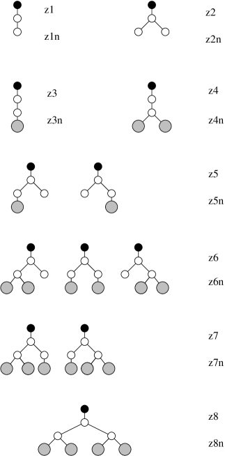
Figure 5: Calculation of $RT_{c}(r=1)$

We have shown that a large class of BP models exhibits a long range negative power like correlations in the canonical ensemble. Those correlations are not finite size effects and survive in the $n\rightarrow\infty$ limit. The shape of those correlations bears a striking resemblance to the shape of correlation functions measured in 4d simplicial gravity [1]. Before making a detailed comparison one should keep in mind that the exact correspondence between the BP and 4d gravity is not known. The quantity measured in [1] has only a qualitative resemblance to the quantity calculated here. We believe however that the same mechanism can be responsible for both.

7 Acknowledgments

I would like to thank Zdzislaw Burda, Jerzy Jurkiewicz and Jan Smit for many helpful discussions and comments. This work is supported by the ’Stichting voor Fundamenteel Onderzoek der Matierie’ (FOM). The numerical simulations were partially carried out on the PowerXplorer at SARA.

Appendix A Calculation of $G(n,t;r)$

The inverse Laplace transform (continuous) of $G(\mu,t;r)$ is given by

$$G(n,t;r)\approx\frac{1}{2\pi i}\int_{c-i\infty}^{c+i\infty}\text{d}\mu G(\mu,t;r)e^{n\mu}$$ (24)

where $c>\mu_{c}$. The saddle point equation is

$$\frac{\partial\log(G(\mu,t;r))}{\partial\mu}=-n.$$ (25)

Using the (4) and (7) we can expand the left hand side of (25). Because we are interested in $n\gg 1$ we keep only the largest term of the expansion (in $\Delta\mu$) of the left hand side of (25). Solving this we obtain

$$\mu_{s}\approx \frac{\left(r\frac{Z_{0}}{Z_{1}}+\frac{1}{2}\frac{Z_{1}}{Z_{0}}\right)^{2}}{n^{2}}+\mu_{c},$$ (26)

$$\begin{split}G(\mu_{s},t;r)\approx&Z_{0}\exp\left[-\frac{1}{n}\left(2\frac{Z_{0}^{2}}{Z_{1}^{2}}r^{2}+2r+\frac{1}{2}\frac{Z_{1}^{2}}{Z_{0}^{2}}\right)\right],\end{split}$$ (27)

$$\frac{\partial^{2}\log(G(\mu_{s},t;r))}{\partial\mu^{2}}\approx \frac{1}{2}\frac{n^{3}}{\left(r\frac{Z_{0}}{Z_{1}}+\frac{1}{2}\frac{Z_{1}}{Z_{0}}\right)^{2}}.$$ (28)

Putting it all together we get the formula (16). Formulas for other two-point functions can be obtained in a similar way.

References

[1]B. V. de Bakker, J. Smit, Nucl. Phys. B454 (1995) 343.
[2]J. Ambjørn, B. Durhuus, J. Fröhlich, P. Orland
Nucl. Phys. B270 (1986) 457.
[3]J. Ambjørn, B. Durhuus, T. Jonsson,
Phys. Lett. B244 (1990) 403.
[4] J. Ambjørn, J. Jurkiewicz,
Nucl. Phys. B541 (1995) 643.