1 Introduction

One of the most exciting challenges in the theoretical physics is to understand gravitational interaction in the context of the quantum theory. The problem we encounter when we try to formulate quantum gravity within ordinary field theory in four dimensions is that we cannot renormalize it perturbatively. If we use lattice regularization, which enables a nonperturbative study, general coordinate invariance is not manifest and whether it is restored in the continuum limit is a crucial problem. One possibility of lattice regularization of quantum gravity is dynamical triangulation, which is believed to restore general coordinate invariance in the continuum limit. It has been solved exactly in two dimensions and its continuum limit is shown to reproduce Liouville theory, in which general coordinate invariance has been treated carefully.

Although four–dimensional dynamical triangulation seems to be difficult to solve analytically, there is no potential barrier in studying it through numerical simulation. Employing the Einstein–Hilbert action as the lattice action and sweeping the gravitational constant, it has been discovered that the system undergoes a second order phase transition [1, 2], which suggests the possibility of taking a continuum limit. One of the main purpose of this paper is to try to clarifying the physical meaning of this phase transition.

When we regularize four–dimensional quantum gravity with dynamical triangulation the integration over the metric is replaced with the random summation over all possible four–dimensional simplicial manifolds.

Although we can modify the lattice action expecting universality, it is natural to start with the Euclidean Einstein–Hilbert action

$$S=\int\mbox{d}^{4}x\sqrt{g}\left(\Lambda-\frac{1}{G}R\right)$$ (1)

as a first trial, where $\Lambda$ is the cosmological constant and $G$ is the gravitational constant. Let us denote the number of $i$-simplices in a simplicial manifold by $N_{i}$. One can easily find that, for a simplicial manifold,

$$\int\mbox{d}^{4}x\sqrt{g} = cN_{4}$$ (2)

$$\int\mbox{d}^{4}x\sqrt{g}R = 2\pi N_{2}-10\alpha N_{4},$$ (3)

where $c$ is the volume of each four–simplex and $\alpha$ is the angle between two faces of a four–simplex, which is equal to $\arccos\left(\frac{1}{4}\right)$. Therefore the Einstein–Hilbert action (1) can be expressed in terms of lattice variables as

$$S_{\mbox{{\scriptsize lat}}}=\kappa_{4}N_{4}-\kappa_{2}N_{2},$$ (4)

where $\kappa_{4}$ and $\kappa_{2}$ are related to $\Lambda$ and $G$ through,

$$\kappa_{4}=c\Lambda+\frac{10\alpha}{G},~{}~{}~{}~{}~{}~{}~{}~{}~{}~{}~{}~{}~{}\kappa_{2}=\frac{2\pi}{G}.$$ (5)

2 The Vertex Order Concentration

We consider an ensemble with a fixed $N_{4}$ and with spherical topology. There are well established methods for generating such an ensemble through numerical simulations, and the technical details of our simulation shall be given elsewhere [3]. Our code is written for arbitrary dimension following Ref. [4].

Let us turn to the results of our simulation. We first look at the second order phase transition, which can be seen through thermodynamic quantities such as the average curvature per unit volume :

$$R_{\mbox{{\scriptsize av}}} = \frac{R_{\mbox{{\scriptsize tot}}}}{N_{4}}~{}~{}~{}(R_{\mbox{{\scriptsize tot}}}=\int\mbox{d}^{4}x\sqrt{g}R)$$ (6)

$$= 2\pi\frac{N_{2}}{N_{4}}-10\alpha.$$ (7)

Fig. 2 shows our results for $\langle R_{\mbox{{\scriptsize av}}}\rangle$ at various $\kappa_{2}$’s.

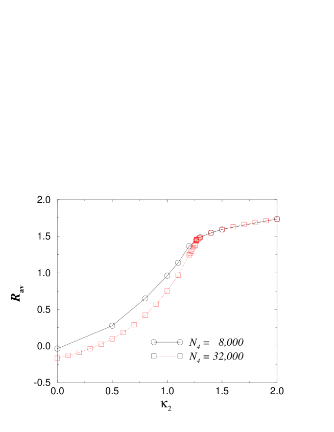
Figure 1: The average curvature per volume is plotted against $\kappa_{2}$ for $N_{4}=8000,32000$.

In contrast to the three–dimensional case [5], no hysteresis has been observed. Also, one sees that the size dependence of the data changes abruptly at $\kappa_{2}=1.2\sim 1.3$. On the right there is little size dependence, whereas on the left, the curve goes lower and lower as we increase the system size. The derivative of the average curvature gives the susceptibility

$$\chi_{R}=2\pi\frac{\partial\langle R_{\mbox{{\scriptsize av}}}\rangle}{\partial\kappa_{2}}=\frac{\langle R_{\mbox{{\scriptsize tot}}}^{2}\rangle-\langle R_{\mbox{{\scriptsize tot}}}\rangle^{2}}{N_{4}},$$ (8)

which represents the fluctuation of the total curvature. As is expected from Fig. 2, the susceptibility has a peak around $\kappa_{2}=1.2\sim 1.3$, which grows higher as the system size is increased. This implies that the correlation length of the local curvature diverges at the critical point [6], where we may hope to take a continuum limit. Since $\kappa_{2}$ corresponds to the inverse of the gravitational constant, as is seen from (5), we call the large $\kappa_{2}$ phase as the weak coupling phase and the small $\kappa_{2}$ phase as the strong coupling phase .

Although this phase transition has been observed by many authors[1, 2], the physical origin of this transition might be not understood clearly.

To clarify it, we measure the vertex order distribution as follows. Let the vertex order $o(v)$ be the number of four-simplices sharing the vertex $v$. Then the vertex order distribution $\rho$ can be defined as

$$\rho(n)\equiv\frac{1}{N_{0}}\langle\sum_{v}\delta_{o(v),n}\rangle.$$ (9)

This quantity is measured every 100 sweeps and averaged over 100 configurations. In order to reduce the fluctuations of the distribution, we smear the data over bins of size 10.

We first note that the average vertex order per one vertex, $\overline{o(v)}$, can be given as

$$\overline{o(v)}\equiv\frac{1}{N_{0}}\sum_{v}o(v)=\frac{5N_{4}}{N_{0}}={10N_{4}\over N_{2}-2N_{4}+4}.$$ (10)

In the second equality, we used the relation $\sum_{v}o(v)=5N_{4},$ which comes from the fact that each four-simplex has five vertices.

From Eq. (4) and Eq. (10), when we move from the strong coupling phase ($\kappa_{2}\sim 0.0$) to the weak coupling phase ($\kappa_{2}\sim 2.0$) with fixed system size, $N_{2}$ increases and thus $\overline{o(v)}$ goes to a smaller value.

In Fig. 2 we show the vertex order distribution $\rho(n)$ for $\kappa_{2}$ = 0.0, 1.267 (near the critical point) and $2.0$ with $N_{4}=32,000$. For $\kappa_{2}=0.0$, one finds that there is an isolated peak of very large vertex order; as large as one third of the total four-simplices.

As $\kappa_{2}$ is increased from 0.0 the position of the peak shifts to left in accordance with the decrease of the $\overline{o(v)}$ and around the critical point ($\kappa_{2}\sim 1.2$) the peak is absorbed into the continuum part of the distribution. For $\kappa_{2}=2.0$, on the other hand, the distribution damps quite rapidly for large vertex order and we have confirmed that it remains almost unchanged when we increase the system size.

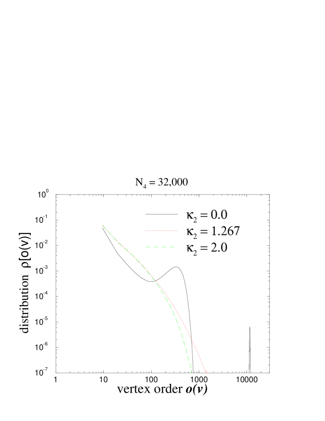
Figure 2: The vertex order distribution for $\kappa_{2}=0,1.267,2.0$ for $N_{4}=32000$.

In Fig. 2 we show the size dependence of the vertex order distribution for $\kappa_{2}=0.0$. One finds that the very large vertex order grows linearly as one increases $N_{4}$, and thus this concentration might be relevant even in the thermodynamic limit.

We call this peculiar phenomenon as the vertex order concentration (VOC). We have also confirmed that the peak consists of two vertices, and we found no link order concentration; there is no singular link shared by conspicuously large numbers of four–simplices.

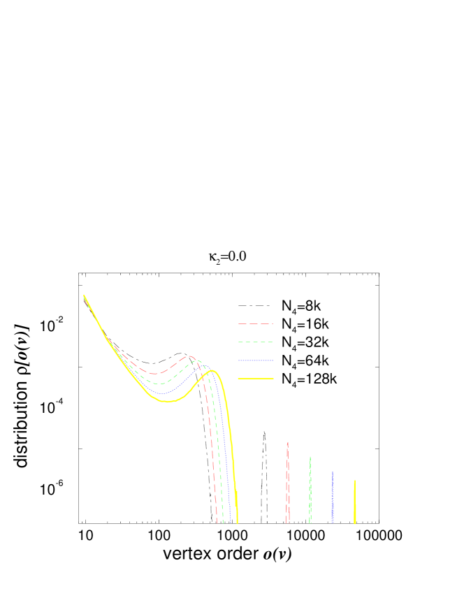
Figure 3: The vertex order distribution for $\kappa_{2}=0$ varying the system size $N_{4}$ from 8k to 128k.

3 The thermalization check

One may suspect that our Monte Carlo simulation is trapped by a local minimum (meta-stable state) and sweeps over only a limited part of the whole configuration space. To check that this suspicion is not the case, we prepare three types of configurations for initial configurations from which we start simulations.

The first one consists of six four-simplices which are the surface of a five-simplex; we call this the hot start configuration. The second one is the cold start, for which we prepare approximately flat configuration, using the surface of the five-dimensional rectangular complex (box). The system size of the cold start configuration can be adjusted near the target number $N_{4}^{0}$ and it has no VOC[3]. The third configuration, four-VOC configuration, has four singular vertices and is made in the following way. We prepare two configurations of system size $N_{4}^{0}/2$ by performing sufficiently many sweeps in strong coupling phase. Each of the thermalized configurations has two singular vertices. Then we identify one four-simplex of one configuration with one four-simplex of the other, so that the resulting manifold is the four-sphere of system size $N_{4}^{0}-1$ with four singular vertices. So this configuration has twice as many singular vertices as the configuration obtained in strong coupling region.

After performing more than 10,000 Monte Carlo sweeps we found no dependence on the three types of initial configurations for any of our observables.

For example, we show the history of the vertex order below. Let us label the vertices of the configuration as $v_{i}$, so that $o(v_{i})\geq o(v_{i+1})$ is satisfied for any $i=1,2\cdots N_{0}$. We show the $o(v_{1})$ (the largest vertex order) as a function of the number of Monte Carlo sweep from each initial configuration together with $o(v_{2})$ and $o(v_{3})$ for $\kappa_{2}=0.0$ in Fig. 3. We only show the results of the simulation for the cold and hot starts for the legibility. For each types of initial configuration (thick curves or thin curves), one can see that there are two large vertex orders $o(v_{1})$ and $o(v_{2})$ around $25,000$ and a large gap between $o(v_{3})$ and the above two. Below the curve of $o(v_{3})$, the curves of $o(v_{i}),i\geq 3$ run closely without significant gaps. One can easily see that the two curves of each $o(v_{i}),i=1,2,3$ are almost identical after 10,000 sweeps.

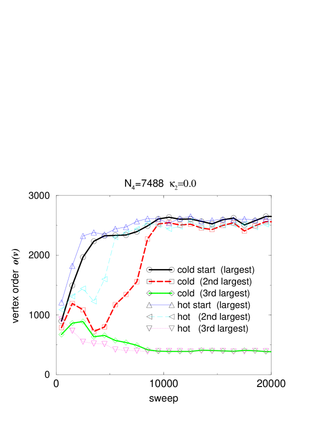
Figure 4: The history of the vertex order for $\kappa_{2}=0$ for the hot and cold initial configurations.

Considering that the vertex order distributions of the three types of configurations are quite different from each other, the above fact strongly suggests that our result, the existence of two singular vertices in strong coupling region, does not come from the insufficiency of thermalization but reflects true properties of the path-integral measure of the dynamical triangulation.

4 The torus topology

We test a possibility of the phenomenon of the VOC being related to the constraint of the topology of the manifold,i.e the manifold must be $S^{4}$. We change the manifold from four-dimensional sphere ($S^{4}$) to the torus ($(S^{1})^{4}$). The method of making the $(S^{1})^{4}$ triangulation is as follows.

1. Prepare the four-dimensional rectangular complex (four-box) and identify each pair of parallel boundary. Draw one line $l_{d}$ between two vertices which is diagonal to each other.

2. Divide the four-boxes into $4!$ four-simplices. The dividing edges on boundaries of the four-boxes must be projections of the diagonal line of $l_{d}$ for consistent construction of the torus triangulation.

For simplicity Fig. 4 describes the three-dimensional case.

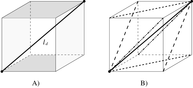
Figure 5: The construction of the torus triangulation.

The resulting triangulation has $(S^{1})^{4}$ topology, from which we start the Monte Carlo simulation.

Fig. 4 shows the comparison of the vertex order distribution $\rho(n)$ between the sphere and the torus case for $N_{4}=128,000$. The $\rho(n)$ of the torus of the size $N_{4}\mathrel{\mathchoice{\lower 0.86108pt\vbox{\halign{$\m@th\displaystyle \hfil#\hfil$\cr<\crcr\sim\crcr}}}{\lower 0.86108pt\vbox{\halign{$\m@th\textstyle \hfil#\hfil$\cr<\crcr\sim\crcr}}}{\lower 0.86108pt\vbox{\halign{$\m@th\scriptstyle \hfil#\hfil$\cr<\crcr\sim\crcr}}}{\lower 0.86108pt\vbox{\halign{$\m@th\scriptscriptstyle \hfil#\hfil$\cr<\crcr\sim\crcr}}}}100,000$ is sensitive to whether the manifold is the torus or the sphere, while for the larger manifold $N_{4}\sim 128,000$ the distribution is almost identical between the two topologies (Fig. 4).

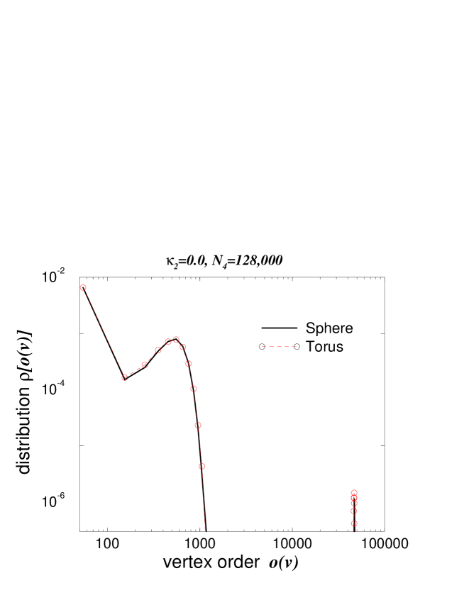
Figure 6: The vertex order distribution of the sphere and the torus. $N_{4}=128,000,\kappa_{2}=0.0$.

The number of the singular vertices in torus manifold is one for $N_{4}\mathrel{\mathchoice{\lower 0.86108pt\vbox{\halign{$\m@th\displaystyle \hfil#\hfil$\cr<\crcr\sim\crcr}}}{\lower 0.86108pt\vbox{\halign{$\m@th\textstyle \hfil#\hfil$\cr<\crcr\sim\crcr}}}{\lower 0.86108pt\vbox{\halign{$\m@th\scriptstyle \hfil#\hfil$\cr<\crcr\sim\crcr}}}{\lower 0.86108pt\vbox{\halign{$\m@th\scriptscriptstyle \hfil#\hfil$\cr<\crcr\sim\crcr}}}}100,000$ and two for $N_{4}\sim 128,000$. From these results we might say that the finite size effect of torus is severer than the sphere case. And the vertex order distribution $\rho(n)$ seems to be almost insensitive to the topology difference, but of course more high statistic simulations of more variation of topology (e.g. $(S^{2})^{2}$, $D^{4}$ etc.) are necessary for the definite conclusions.

5 Discussion

To summarize, we found two singular vertices in the strong coupling region, which disappear in weak coupling region. Although the thermalization is checked, the existence of this VOC is still very strange. The VOC in $\kappa_{2}=0$ case, for which we observe purely the measure of path integral without any weight from the action, implies that the number of such VOC configuration is much larger than the number of the smooth (non VOC) configuration in dynamical triangulation. Such a singular behavior might be an obstacle to the continuum limit. Considering universality in quantum gravity, as well as in ordinary field theories, we think that a sound second order phase transition without VOC, where we can take a sensible continuum limit, should be searched by modifying the lattice action[7, 2, 3] to suppress the VOC.

Acknowledgements.

Numerical calculations for the present work have been performed on HP-700 series at KEK and Univ. of Tokyo. We would like to thank Prof. H. Kawai, Prof. T. Yukawa and Dr. N. Tsuda for stimulative discussions. This work is supported in part by the Grants-in-Aid of the Ministry of Education.

References

-
[1]
J. Ambjørn and J. Jurkiewicz, Phys. Lett. B278 (1992)
42.
M.E. Agishtein and A.A. Migdal, Mod. Phys. Lett. A7 (1992) 1039; Nucl. Phys. B385 (1992) 395, hep-lat/9204004.
S. Varsted, Nucl. Phys. B412 (1994) 406.
B. V. de Bakker and J. Smit, Phys. Lett. B334 (1994) 304, hep-lat/9405013.
S. Catterall, J. Kogut and R. Renken, Phys. Lett. B328 (1994) 277,hep-lat/9401026. - [2] B. Brügmann, Phys. Rev. D47 (1993) 3330, hep-lat/9210001. B. Brügmann and E. Marinari, Phys. Rev. Lett. 70 (1993) 1908, hep-lat/9210002.
- [3] T. Hotta, T. Izubuchi and J. Nishimura, Prog. Theor. Phys. 94 (1995) 263.
- [4] S. Catterall, Comput. Phys. Commun. 87(1995) 409, hep-lat/9405026.
-
[5]
J. Ambjørn, D.V. Boulatov, A. Krzywicki and S. Varsted,
Phys. Lett. B276 (1992) 432.
J. Ambjørn and S. Varsted, Nucl. Phys. B373 (1992) 557. -
[6]
J. Ambjørn and J. Jurkiewicz,
“Scaling in four dimensional quantum gravity”,
NBI-HE-95-05, February 1995, hep-th/9503006.
B.V. de Bakker and J. Smit, “Two–point functions in 4D dynamical triangulation”, ITFA-95-1, March 1995, hep-lat/9503004. -
[7]
J. Ambjørn, J. Jurkiewicz and C.F. Kristjansen,
Nucl. Phys. B393 (1993) 601, hep-th/9208032.