Analysis of Hadron Propagators with One Thousand Configurations on a $24^{3}\times 64$ Lattice at $\beta=6.0$

Abstract

Statistical properties of effective mass are analyzed. We show from a general ground that effective mass as a function of time should not exhibit long plateaux whatever high statistics simulations are made: the mass should fluctuate beyond the one standard deviation of error bars after a few time slices for large times where the ground state dominates. This explains the difficulty of obtaining long plateaux experienced in previous simulations. Implications of the observation for global $\chi^{2}$ fits are discussed, and results for hadron masses are presented.

1 Introduction

Calculation of hadron masses constitutes a basic part in virtually all problems of lattice QCD simulations. A quantity always examined in such calculations is the effective mass $m_{\rm eff}(t)$. The existence of a plateau in $m_{\rm eff}(t)$ as a function of time $t$ is regarded as a dual measure for the statistical quality of data and the minimum time separation beyond which the ground state dominates. In this way the plateau is used as a guide in the choice of the time interval for a global $\chi^{2}$ fitting to extract hadron masses from propagators. In practice, however, a long plateau has rarely been seen. Even in the best previous efforts toward high statistics simulations[1, 2, 3, 4], effective masses, particularly for $\rho$ meson and the nucleon, almost always deviate from a plateau beyond error bars after 5 or 6 times slices. Ensuing uncertainties in the choice of the fitting range and fitted values of hadron masses have represented a severe hindrance factor in attempts toward high precision determination of hadron masses, especially for light hadrons[5].

In this report we present an analysis on the origin of this problem. Our study is based on hadron propagators for the Wilson quark action at $K=0.1545,0.1550,0.1555$ evaluated on 1000 quenched gauge configurations on a $24^{3}\times 64$ lattice at $\beta=6.0$, which were generated with the 5-hit pseudoheatbath algorithm at 2000 sweep intervals. The central value $K=0.1550$ has been chosen to facilitate a comparison with previous high statistics studies[1, 2, 4] which employ up to 400 configurations for the same spatial size[2] or a larger size of $32^{3}$[4].

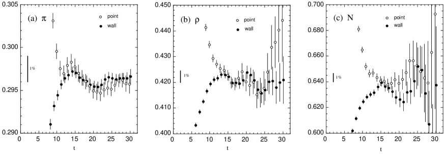
Figure 1: Effective mass for (a) $\pi$, (b) $\rho$ and (c) $N$ at $\beta=6.0$ and $K=0.1550$ on a $24^{3}\times 64$ lattice with 1000 configurations. Errors are estimated by a single elimination jackknife procedure.

This calculation is one of the first QCD runs carried out by the JLQCD Collaboration on VPP500/80 at KEK which started operation in January 1995. The machine consists of 80 processing elements (PE’s), each with the peak speed of 1.6GFLOPS and 256MBytes of memory, connected by a crossbar switch. Our run used 64 processors, on which our code for heatbath and red/black minimal residual solver sustained the speed of $1.0-1.3$ GFLOPS/PE. The configuration generation of 2000 sweeps and a calculation of standard meson and baryon propagators for the point and wall sources on the final configuration was made in about 30 minutes, so that the entire run took about 20 days to complete.

2 Analysis of effective mass

In Fig. 1 we show the effective mass for $\pi$, $\rho$ and nucleon ($N$) obtained with the point(open circles) or the wall (filled circles) source at $K=0.1550$ or $m_{\pi}/m_{\rho}\approx 0.7$, which roughly corresponds to strange quark mass. A striking feature observed in these plots is the presence of fluctuations which exceed the level of one standard deviation after a few time slices even for $\pi$ and with 1000 configurations.

In fact it is possible to understand this behavior by a simple statistical analysis. To show this, let $\overline{G(t)}$ be the average for a hadron propagator over $N$ independent configurations, and $G_{\rm true}(t)=\langle G(t)\rangle$ be the true propagator. According to the central limit theorem, the difference $\delta G(t)=\overline{G(t)}-G_{\rm true}(t)$ obeys the distribution,

$$P[\overline{G}]\propto\exp\left[-\frac{N}{2}\sum_{t,t^{\prime}}\delta G(t)C^{-1}(t,t^{\prime})\delta G(t^{\prime})\right],$$ (1)

where the covariance matrix $C$ is defined by

$$C(t,t^{\prime})=\langle G(t)G(t^{\prime})\rangle-\langle G(t)\rangle\langle G(t^{\prime})\rangle.$$ (2)

Let us introduce a normalized covariance matrix

$$\tilde{C}(t,t^{\prime})\equiv\frac{C(t,t^{\prime})}{\sqrt{C(t,t)C(t^{\prime},t^{\prime})}}$$ (3)

and denote the eigenvalues and normalized eigenvectors of $\tilde{C}(t,t^{\prime})$ by $\lambda_{i}$ and $e_{i}(t)$ $(i=1,\cdots,L_{t})$ with $L_{t}$ the temporal lattice size. An eigenvector decomposition of the averaged propagator leads to the formula,

$$\overline{G(t)}=G_{\rm true}(t)+\sqrt{\frac{C(t,t)}{N}}\sum_{i=1}^{L_{t}}\sqrt{\lambda_{i}}e_{i}(t)\xi_{i},$$ (4)

where, according to (1), $\xi_{i}\,(i=1,\cdots,L_{t})$ are independent Gaussian random numbers.

Figure 2: Four examples of effective mass for $\pi$ (top row) and $\rho$ (bottom row) for point source calculated from “simulated” propagators (solid curves) as compared to the measured values for $K=0.1550$ (shown with error bars) taken from Fig. 1. Dotted lines correspond to the model (5).

Given a model of the true propagator $G_{\rm true}(t)$ and a measured value of the covariance matrix, this formula allows us to generate “simulated” samples of the averaged propagator $\overline{G(t)}$ by generating a set of $L_{t}$ Gaussian random numbers $\xi_{i}$.

For the model of $G_{\rm true}(t)$ we take a double hyperbolic cosine form,

$$G_{\rm true}(t)=Ze^{-mt}+Z^{\prime}e^{-m^{\prime}t}+(t\to L_{t}-t),$$ (5)

where the masses and residues are determined by a $\chi^{2}$ fit of the measured propagator over $6\leq t\leq L_{t}/2$. In Fig. 2 we show four examples of effective mass for $\pi$ and $\rho$ for the point source calculated from “simulated” propagators (solid curves). Dotted lines represent values for the model (5). These examples clearly demonstrate that fluctuations as observed in Fig. 1 are a typical occurrence. Indeed some of the examples are amusingly similar to the measured value.

Let us add a remark that the diagonal of the covariance matrix is expected to behave as $C(t,t)\propto\exp(-\alpha t)$ with $\alpha=2m_{\pi}$ for $\pi$ and $\rho$ and $\alpha=3m_{\pi}$ for $N$[6], with which our data are consistent. Combined with (4) this explains why the magnitude of fluctuation of $m_{\rm eff}$ increases rapidly for $\rho$ and $N$ toward large times, while it stays roughly constant for $\pi$.

We now reexamine the concept of a plateau in the light of the above analysis. Let us define a plateau over the time interval $t_{1}\leq t\leq t_{2}$ by the condition that $m_{\rm eff}(t)$ over this interval falls within a band of width $2\delta m$ centered at $m$, i.e., $m-\delta m\leq m_{\rm eff}(t)\leq m+\delta m$ for $t=t_{1},\cdots,t_{2}$. To calculate the probability for the occurrence of such a plateau, we make a change of variable $P[\overline{G}]\to P[m_{\rm eff}(t_{1}),\cdots,m_{\rm eff}(t_{2})]$ in (1), defining $m_{\rm eff}(t)=\log\overline{G(t)}/\overline{G(t+1)}$ (effects of the periodic boundary condition are small in the numerical results below). The probability is then given by an integral of $P[m_{t_{1}},\cdots,m_{t_{2}}]$ over $m-\delta m\leq m_{t_{i}}\leq m+\delta m(i=t_{1},\cdots,t_{2})$.

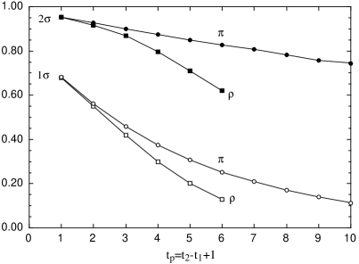
Figure 3: Probability for plateau of length $t_{p}$ starting at $t_{1}=15$ for $\pi$ and $\rho$. Open and filled symbols correspond to the choice of $\delta m$ equal to one or two standard deviations of $m_{\rm eff}(t_{1}=15)$.

In Fig. 3 we plot the probability of finding a plateau of length $t_{p}(=t_{2}-t_{1}+1)$ for $\pi$ and $\rho$ calculated with the measured covariance matrix for $K=0.1550$ for the case of the wall source. We fix $t_{1}=15$, since we have chosen the ground state mass $m$ by a $\chi^{2}$ fit with a single hyperbolic cosine over $15\leq t\leq L_{t}/2$. For $\delta m$ we choose one (open symbols) or two (filled symbols) standard deviation of $m_{\rm eff}(t)$ at $t=t_{1}$. Values for $\rho$ for $t\geq 7$ are not shown because of the poor quality of the covariance matrix for large times.

This figure shows that one should not expect to see a plateau at the level of one standard deviation even for $\pi$: the probability drops below 50% after 2 time slices. Allowing for a deviation of two standard deviations, a plateau of length 10 for $\pi$ ($3-4$ units in terms of the correlation length $\xi_{\pi}=1/m_{\pi}$) becomes probable, while for $\rho$ the probability decreases to $60-50$% already at $t\approx 6-7$ ($t/\xi_{\rho}\approx 3$). These features are consistent with actual examples of effective mass shown in Fig. 1, and also with those of previous high statistics simulations[1, 2, 3, 4].

We should emphasize that the pattern of fluctuations of effective mass does not change when one increases the number of configurations $N$, except that the magnitude scales down as $1/\sqrt{N}$. At the same time statistical errors estimated for $m_{\rm eff}$ also decreases as $1/\sqrt{N}$. In this sense higher statistics does not lead to a longer or better plateau. In other words we can ask for such an improvement only within a fixed magnitude of the absolute error (e.g., 1% of mass). Let us add that the use of larger spatial volumes and improved operators having a larger coupling to the ground state also help to obtain a better plateau only in the latter sense.

3 $\chi^{2}$ fits for hadron masses

Table 1: Hadron masses in lattice units at $\beta=6.0$. For our results and those of QCDPAX the first and second row correspond to point and wall source. APE used multi-origin $7^{3}$ source, while LANL results are combined estimates from wall and Wuppertal-smeared source.

$\quad K$	$\quad\pi$	$\quad\rho$	$\quad N$
0.1545	0.33075(40)	0.4441(6)	0.6828(21)
	0.33076(28)	0.4425(10)	0.6777(21)
0.1550	0.29642(42)	0.4231(16)	0.6451(11)
	0.29642(27)	0.4220(12)	0.6393(27)
0.1555	0.25867(46)	0.4019(20)	0.6066(13)
	0.25864(33)	0.4016(17)	0.6003(37)
Previous results at $K=0.1550$
APE	0.298(2)	0.429(3)	0.647(6)
QCDPAX	0.2960(8)	0.4201(29)	0.6403(50)
	0.2964(6)	0.4228(19)	0.6307(39)
LANL	0.297(1)	0.422(3)	0.641(4)

Our analysis should have made it clear that restricting the fitting range of a global $\chi^{2}$ fit to the time interval of an apparent plateau is not well founded. In fact if one repeats a simulation with a different sequence of random numbers the effective mass will generally exhibit a plateau at some other time interval at a different value. This indicates that it is more reasonable to take the minimum time $t_{min}$ at the time slice where the dominance of the ground state is reasonably ensured (e.g., by the overlap of $m_{\rm eff}$ for the point and wall sources), and to extend the fitting range to large times as long as statistical fluctuations do not become unacceptably large, without resorting to the presence of plateau. The value of correlated $\chi^{2}$ should tell whether the choice is reasonable. Of course the fitted values of hadron masses vary depending on the choice of the interval. However, this is an uncertainty which can only be reduced by an improved measurement of hadron propagators.

In Table 1 we present hadron masses obtained by a correlated $\chi^{2}$ fit over the interval $15\leq t\leq L_{t}/2=32$ with a single hyperbolic cosine for $\pi$ and $\rho$ and with a single exponential for $N$. Errors correspond to an increase of $\chi^{2}$ by one. For $\pi$ and $\rho$ our results obtained with the point and wall sources are mutually in agreement. For $K=0.1550$ previous results from the QCDPAX Collaboration[2] and from the Los Alamos group[4] are consistent with ours, while those from APE are higher. The case of nucleon is problematical. We find that the $\chi^{2}$ fit is not very stable and that the point and wall results do not agree within the error. Effort toward improving baryon operators will be needed for a precise determination of baryon masses even in the region of strange quark.

References

- [1] S. Cabasino et al., Phys. Lett. B258 (1991) 195.
- [2] Y. Iwasaki et al., Nucl. Phys. B(Proc. Suppl.)34 (1994) 354.
- [3] F. Butler et al., Nucl. Phys. B430 (1994) 179.
- [4] T. Bhattacharya and R. Gupta, Nucl. Phys. B(Proc. Suppl.)42 (1995) 935.
- [5] A. Ukawa, Nucl. Phys. B(Proc. Suppl.)30 (1993) 3.
- [6] See, e.g., G. P. Lepage, in Proc. of TASI ’89 (World Scientific, 1990), p. 97.