Hypercubic Smeared Links for Dynamical Fermions

Abstract

We investigate a variant of hypercubic gauge link smearing where the $SU(3)$ projection is replaced with a normalization to the corresponding unitary group. This smearing is differentiable and thus suitable for use in dynamical fermion simulations using molecular dynamics type algorithms. We show that this smearing is as efficient as projected hypercubic smearing in removing ultraviolet noise from the gauge fields. We test the normalized hypercubic smearing in dynamical improved (clover) Wilson and valence overlap simulations.

I Introduction

In recent years, significant progress has been made in full QCD lattice simulations. There are simulations with 2+1 flavors, with realistic quark masses, and in large volumes, though frequently only two of the three conditions are met at once. These simulations are performed with different kinds of fermion formulations, from the simplest unimproved Wilson fermions to highly improved nearly chiral fermions, with improved rooted staggered fermions and even with the expensive but exactly chiral overlap fermions. All these calculations, even those with inexact chiral symmetry, are still expensive and require large computer resources. Improving the fermionic action such that simulations could be performed on coarser lattices, or improving the performance of algorithms to better fit today’s computer power is important for truly realistic simulations. It seems that a simple modification, the use of smeared gauge fields in the fermionic action, can help improve both the action and the computational performance as well.

Smeared links are a natural part of improved fermionic actions. In the perfect action formulation the Dirac operator at the renormalization group fixed point is fitted by an extended but ultra-local Dirac operator. This fit is not feasible unless the gauge links of the Dirac operator are smeared Hasenfratz et al. (2002a). The exactly chiral overlap operator Neuberger (1998) effectively also contains smeared links, even if the kernel operator is based on thin links. This can be seen when one considers the expanded form of the overlap formulation with the square root term in $d(-R_{0})/\sqrt{d^{\dagger}(-R_{0})d(-R_{0})}$. The order $d^{3}$, $d^{5}$, etc. terms all contribute to the nearest neighbor fermion coupling of the overlap Dirac operator with extended gauge connections. The most frequently used staggered fermion formulation, the so called Asqtad action, also uses fat links Orginos et al. (1999). The smeared links discussed above are part of the definition of the Dirac operator. The gauge action is independent and in most cases is not smeared.

The effect of smearing is two-fold. First, it averages out small scale vacuum fluctuations, reducing the non-physical ultra-violet noise in the fermionic action, secondly it removes extreme local fluctuations of the gauge fields, lattice dislocations. In the various fermion discretizations, the effect of vacuum fluctuations and dislocations comes in different disguises. Staggered fermions’ taste breaking is triggered by gauge field fluctuations within the hypercube and smearing can effectively reduce this effect Orginos et al. (1999); Hasenfratz and Knechtli (2001). For Wilson fermions dislocations contribute to the spread of the near zero real modes of the Dirac operator. Those modes make it impossible to simulate at small quark masses without going to very fine lattice spacing, and/or large volumes Del Debbio et al. (2006). Smearing removes the dislocations and reduces the spread of the eigenmodes DeGrand et al. (1999).

Chiral fermions can also benefit from smeared links. The cost of the overlap operator is largely given by the density of low modes of the kernel operator from which it is constructed. Smearing reduces the occurrence of these low modes and thereby can reduce the cost of applying the operator by an order of magnitude DeGrand and Schaefer (2005a, b). In simulations using domain wall fermions, the low modes of the kernel operator are known to cause explicit breaking of chiral symmetry, indicated by a non-vanishing residual mass. If there are fewer of those modes, chiral symmetry is realized to a higher degree and one can use a smaller fifth dimension without increasing the residual mass.

There is no unique criterion what constitutes a “good” smearing procedure besides the explicit construction of the fixed point Dirac operator or the expanded form of overlap fermions. Without such guiding principles, any smearing, as long as it consists of adding irrelevant (local) operators to the action, is acceptable. The smeared links do not even have to be $SU(3)$ elements as is illustrated by the success of the Asqtad action. Any acceptable procedure will lead to a valid action, but chosen properly, smearing will improve the scaling of the continuum limit. If the modification of the gauge fields are too weak, the smearing has no effect. On the other hand, a definition of the fat link which spreads over many sites and heavily mixes the links can lead to an action which again has strong cut-off effects DeGrand et al. (2003). Thus, an optimal smearing is as local as possible while removing as much of the short scale fluctuations as possible.

The first smearing was introduced by the APE collaboration Albanese et al. (1987) and different forms of smearing have been used in quenched studies since then. Dynamical simulations with smeared links became practical when the fully differentiable stout smearing was proposed by Morningstar and Peardon Morningstar and Peardon (2004). Iterating either APE or stout links can wash out short to intermediate scale physical properties of the action, leading to large scale violations in quantities sensitive to those scales. Hyper-cubic (HYP) blocking, introduced in Ref. Hasenfratz and Knechtli (2001), circumvents this problem by reducing the spread of consecutive smearing steps. In this paper, we will discuss variants of the HYP blocking that are differentiable and suitable for molecular dynamics simulations.

In the next Section we first modify the APE construction by replacing the original $SU(3)$ projection by a normalization to $U(3)$. These normalized n-APE links are differentiable and as effective in removing short scale vacuum fluctuations as the projected APE smearing. Next we combine n-APE smearing with the HYP definition and show that n-HYP links are as effective as 3 levels of stout smearing and are considerably better than HYP links constructed from stout smearing. The differentiable n-HYP smearing can be used in dynamical simulations and in Sect. III we give details of how the fermionic force can be evaluated with n-HYP smearing. This force term can be combined with any fermionic action and in Sect. IV we illustrate the effectiveness of the smearing both with overlap and Wilson clover fermions.

II Definition of the smeared links

The APE smeared link Albanese et al. (1987) is the basis of most smearing methods. First the staple sum $\Gamma_{n,\mu}=\sum_{\nu\neq\mu}U_{n,\nu}U_{n+\nu,\mu}U_{n+\mu,\nu}^{\dagger}$ is added to the original link $U_{n,\mu}$ as

$$\Omega_{n,\mu}=(1-\alpha)U_{n,\mu}+\alpha^{\prime}\,\Gamma_{n,\mu}\;.$$ (1)

Here $\alpha^{\prime}=\alpha/m$ and $m$ is the number of staples included in the staple sum. Next $\Omega$, a general $N\times N$ matrix, is projected back to $SU(N)$ as

$$V_{p}={\displaystyle\max_{V\in SU(3)}}\,\textrm{Re tr }(V\Omega^{\dagger})\,.$$ (2)

In the following we will refer to this construction as projected- or p-APE. Since no closed form for the derivative of the p-APE links is known, they are difficult to use in molecular dynamics (MD) simulations.

Not long ago Peardon and Morningstar suggested a differentiable smearing method Morningstar and Peardon (2004). Their construction uses the staple sum $\Gamma_{n,\mu}$ to define the differentiable $SU(N)$ stout link as

$$V_{s} = e^{\rho S}U,$$ (3)

$$S = \frac{1}{2}(\Gamma U^{\dagger}-U\Gamma^{\dagger})-\frac{1}{2N}{\rm tr}(\Gamma U^{\dagger}-U\Gamma^{\dagger})\,.$$ (4)

It is not obvious why the suggested form is a smearing at all beyond the perturbative regime where $\Gamma U^{\dagger}\approx n\,\mathbb{I}$. There the stout links are indeed identical to projected APE smeared links with $\rho=\alpha/6$ Capitani et al. (2006). Nevertheless stout smearing appears to work similarly to APE well beyond the perturbative regime.

Here we consider a smeared link that is closer in spirit to the projected APE links but it is differentiable and appropriate for MD simulations. From the $N\times N$ general $\Omega$ matrix of Eq. (1) we form a $U(N)$ unitary matrix as

$$V_{n}=\Omega(\Omega^{\dagger}\Omega)^{-1/2}\,.$$ (5)

Since $\Omega^{\dagger}\Omega$ is Hermitian and positive definite, $(\Omega^{\dagger}\Omega)^{-1/2}$ is well defined, unless $\mathrm{det}\,\Omega=0$. The smeared link $V_{n}$ is unitary but not in $SU(N)$, its determinant in general is not one. The form in Eq. (5) was first used in Ref. Liang et al. (1993) to define smeared operators, while in Ref. Zanotti et al. (2002) $V_{n}$ is divided by the cube-root of its determinant to define an $SU(N)$ link.

One should note that there is no requirement that the smeared link be an $SU(N)$ element, but in practice projecting the link back to $SU(N)$ was found to be more effective in removing short scale fluctuations. Here we will show that the $U(N)$ element $V_{n}$ link is as effective as the projected smeared link. In the following we will refer to the $V_{n}$ links defined in Eq. (5) as normalized- or n-APE smearing. Since at the 1-loop perturbative level neither the projection nor the normalization of the link plays any role, the 1-loop perturbative properties of all three smearing prescriptions are identical.

HYP smearing, as introduced in Ref. Hasenfratz and Knechtli (2001), consists of three consecutive projected APE type smearing steps but the staple sums at the higher level are constructed such that only links within the hypercubes attached to the original link enter. The consecutive smearing levels are constructed as

$$V_{n,\mu} = \textrm{Proj}_{SU(3)}[(1-\alpha_{1})U_{n,\mu}+\frac{\alpha_{1}}{6}\sum_{\pm\nu\neq\mu}\widetilde{V}_{n,\nu;\mu}\widetilde{V}_{n+\hat{\nu},\mu;\nu}\widetilde{V}_{n+\hat{\mu},\nu;\mu}^{\dagger}]\,,$$ (6)

$$\widetilde{V}_{n,\mu;\nu} = \textrm{Proj}_{SU(3)}[(1-\alpha_{2})U_{n,\mu}+\frac{\alpha_{2}}{4}\sum_{\pm\rho\neq\nu,\mu}\overline{V}_{n,\rho;\nu\,\mu}\overline{V}_{n+\hat{\rho},\mu;\rho\,\nu}\overline{V}_{n+\hat{\mu},\rho;\nu\,\mu}^{\dagger}]\,,$$ (7)

$$\overline{V}_{n,\mu;\nu\,\rho} = \textrm{Proj}_{SU(3)}[(1-\alpha_{3})U_{n,\mu}+\frac{\alpha_{3}}{2}\sum_{\pm\eta\neq\rho,\nu,\mu}U_{n,\eta}U_{n+\hat{\eta},\mu}U_{n+\hat{\mu},\eta}^{\dagger}]\,.$$ (8)

The $U_{n,\mu}$ are the thin links from site $n$ in direction $\mu$, the $V_{n,\mu}$ are the resulting HYP blocked fat links. The intermediate fields $\widetilde{V}$ and $\overline{V}$ are constructed such that the contributions to $V$ are restricted to the attached hyper-cube. The indices after the semi-colon always indicate the directions excluded from the sums. The three SU(3) projections make the HYP smeared configurations very smooth while keeping the smearing within a hypercube ensures that even short distance properties of the configurations are only minimally distorted. While the main ingredient, the SU(3) projections, make the HYP links difficult to use in dynamical simulations, any of the above discussed differentiable smearings can be combined with the HYP construction. In the following we will refer to the original HYP links as p-HYP, to the normalized smearing as n-HYP and the stout HYP construction as stout - or s-HYP. Again, at the 1-loop perturbative level the three descriptions are identical Capitani et al. (2006).

II.1 Stout and n-APE smearing in SU(2)

The two smearing prescriptions are easiest to compare for the gauge group SU(2). The relevant quantity for both is $\Gamma U^{\dagger}$ which is a linear combination of SU(2) elements and can be written as

$$\Gamma U^{\dagger}=\omega_{0}\mathbb{I}+i\,\bar{\omega}\bar{\sigma,}$$ (9)

where $\omega_{0}$ and $\bar{\omega}=\hat{n}\omega$ are real. For $SU(2)$ the traceless anti–Hermitian part of $\Gamma U^{\dagger}$, $S$ in Eq. (4), is just $i\bar{\omega}\bar{\sigma}$ and we thus have

$$V_{s}=e^{i\rho\bar{\omega}\bar{\sigma}}U=[\cos(\rho\omega)+i\,\sin(\rho\omega)\,\hat{n}\bar{\sigma}]U,$$ (10)

while the APE link (1), normalized according to Eq. (5) is

$$V_{n} = \Big{[}\frac{1+\xi\omega_{0}}{N_{0}}+i\frac{\xi\omega}{N_{0}}\hat{n}\bar{\sigma}\Big{]}U\,,$$ (11)

$$N_{0} = \sqrt{(1+\xi\omega_{0})^{2}+(\xi\omega)^{2}}\,,$$ (12)

where $\xi=\alpha^{\prime}/(1-\alpha)$. The stout link is independent of $\omega_{0}$, the trace of $\Gamma U^{\dagger}$, and thus contains less information about the original fields than the n-APE link.

Eqs. (10) and (11) can nevertheless be approximately identical if $\rho\omega,\;\xi\omega\ll 1$, and $\omega_{0}$ can be replaced by its average value. According to Eq. (9) $\omega_{0}$ is related to the trace of the plaquettes around the thin link $U$, so $\langle\omega_{0}\rangle=m\,{\rm tr}(U_{{\rm{plaq}}})/N=m+O(\omega^{2})$ when $\omega\ll 1$. These conditions are satisfied near the continuum limit where fluctuations are suppressed and the gauge links are close to the unit matrix. Then stout and n-APE links agree if $\xi\omega/N_{0}\approx\sin(\rho\omega)$, or

$$\rho=\frac{\xi}{1+\xi\langle\omega_{0}\rangle}=\frac{\alpha/m}{1-\alpha(1-{\rm tr}(U_{{\rm{plaq}}})/N)}\,.$$ (13)

This relation agrees with the perturbatively expected form $\rho=\alpha/m$ if ${\rm tr}(U_{{\rm plaq}})=N$. On typical MC configurations the plaquette is considerably smaller than that, suggesting that even if stout and n-APE smearing can be matched on MC configurations, the corresponding stout parameter could be significantly different from the perturbatively expected value. While the optimal parameter for APE smearing is largely independent of the gauge coupling, this is not so for stout smearing. On rough configurations where $\rho\omega$ is not small and $\omega_{0}$ cannot be replaced by its average, stout links could be very different from n- or p-APE links and resemble little the form of Eq. (1).

II.2 Comparing projected, normalized and stout smearings

Smearing reduces lattice artifacts by removing some of the non-physical ultraviolet fluctuations of the gauge configurations. The effectiveness of the smearing can be measured by the smoothness of the plaquette, i.e. by the value of the average plaquette, and even more so by the distribution of the smallest plaquette on finite volume configurations.

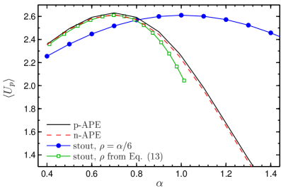
Figure 1: The average plaquette on quenched $\beta=5.8$ configurations as a function of the smearing parameter $\alpha$ after various single level smearings.

The comparisons presented in this section are based on a set of 500 quenched $8^{4}$ lattices generated with the plaquette gauge action at $\beta=5.8$, corresponding to a lattice spacing of 0.136 fm. In Fig. 1 we show the average plaquette after one level of p-APE, n-APE and stout smearing as a function of the smearing parameter $\alpha$. The values measured after projected and normalized APE smearing are nearly indistinguishable, predicting the best smearing at about $\alpha=0.75$. Above this value the smearing becomes unstable, the average plaquette drops even with only one level of smearing. The stout smeared plaquette is plotted in two different ways: once with the perturbatively predicted relation $\alpha=6\rho$, and also with the relation based on the $SU(2)$ prediction of Eq. (13). While the former parametrization leads to a very different result than the APE smeared links, the latter one is surprisingly consistent with those .

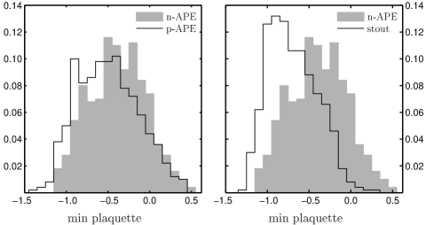
Figure 2: The histograms show the distribution of the smallest smeared plaquette. The left panel compares projected (lines) and normalized (shaded) APE with $\alpha=0.75$ smearing parameter. The right panel compares n-APE (shaded) with $\alpha=0.75$ and stout smearing with $6\rho=1.1$ (lines).

The most extreme fluctuations can be studied from the tail distribution of the plaquette. Figure 2 shows the histogram of the smallest plaquettes. The left panel compares p-APE and n-APE smearings at the same $\alpha=0.75$ parameter value. It is surprising how small the deviation is between the two smearings even here when individual plaquettes are considered. If any difference is observable, it is to the advantage of the n-APE smearing in the sense that the latter produces slightly larger minimal plaquette values. The right panel compares $\alpha=0.75$ n-APE and stout smearing at its optimal value, $6\rho=1.1$. The difference is obvious, n-APE removes more of the extreme fluctuations than stout smearing. Stout smearing with $6\rho=0.75$ is considerably worse than n-APE smearing.

Next we consider HYP links based on the three different smearings. In Ref. Hasenfratz and Knechtli (2001) the projected-HYP parameters were optimized by maximizing the smallest plaquette on a set of coarse ($\beta=5.7$) configurations. The optimal parameters found that way ($\alpha_{1}=0.75,$ $\alpha_{2}=0.6$ and $\alpha_{3}=0.3$) turned out to be fairly independent of the gauge coupling and close to the perturbative values that minimize taste violations for staggered fermions ($\alpha_{1}=0.875$ $\alpha_{2}=0.571$ and $\alpha_{3}=0.25$). Since we found that n- and p-APE smearing are nearly identical numerically and they are identical perturbatively, we expect that the same parameter values are optimal for n-HYP as well. To optimize the stout-HYP parameters we repeated the procedure of Ref. Hasenfratz and Knechtli (2001). We found it difficult to identify an optimal parameter set, the sensitivity, especially to the last parameter $\rho_{3}$, is weak compared to statistical fluctuations. The best parameter values were large, even larger than what one would predict based on Eq. (13), and did not remove as many of the small plaquettes as n-HYP smearing.

In Table 1 we compare the average plaquette and the average of the minimum plaquette values. In addition to n-HYP smearing with parameters $\alpha=(0.75,\,0.6,\,0.3)$ we consider 1, 2 and 3 levels of stout smearing with $6\rho=0.9$ smearing parameter, s-HYP smearing with parameters $6\rho=(0.85,\,0.75,\,0.35)$ and with parameters $6\rho=(1.2,\,1.0,\,0.4)$. The former s-HYP parameters correspond to n-HYP parameters rescaled according to Eq. (13), the latter one to the values found by optimizing the minimum plaquette distribution. The average plaquette value does not always follow the minimum plaquette. Based on the average plaquette one would expect that 2 levels of stout smearing are about the same or better than n-HYP. This expectation is false as we will show in Sect. IV . The minimum plaquette is a much better indicator of the quality of smearing. That observable puts n-HYP close to 3 levels of stout and considerable better than s-HYP even with the optimized b) parameter set.

Smearing	$\,\,\langle{\rm tr}U_{p}\rangle\,\,$	$\,\langle{\rm tr}U_{p}^{{\rm min}}\rangle\,$
$1\times$ stout	2.60	-0.78(1)
$2\times$ stout	2.84	-0.16(2)
$3\times$ stout	2.91	0.46(3)
s-HYP  a)	2.80	-0.39(2)
s-HYP  b)	2.64	0.00(5)
n-HYP	2.82	0.38(3)

Table 1: Comparison of the plaquette and the minimum plaquette values. The different smearings considered are: 1, 2 and 3 levels of stout smearing with $6\rho=0.9$; stout-HYP a) with parameters $6\rho=(0.85,\,0.75,\,0.35)$ ; b) with parameters $6\rho=(1.2,\,1.0,\,0.4)$; n-HYP with standard HYP parameters $\alpha=(0.75,\,0.6,\,0.3)$;

To summarize our observations, we expect normalized-HYP to be as good as projected-HYP with the same parameter values. The n-HYP parameters do not have to be changed with the gauge coupling and perturbative corrections are expected to be small. If stout-HYP smearing is used in numerical simulations, the parameters will have to be tuned depending on the gauge coupling. Stout-HYP smearing with parameters tuned that way is effective in removing average fluctuations though it does not work as well in removing the extreme fluctuations. At one-loop perturbation theory all three smearings are identical, but since the optimal stout parameters at large or moderate lattice spacing are well above the perturbative values, one expects larger perturbative corrections for stout links. In dynamical updates the computational overhead for n-HYP and stout-HYP is similar, therefore overall n-HYP appears to be a better choice for simulations. In the following we describe the implementation of n-HYP smearing in dynamical simulations.

III Force of the NHYP link

The equations of motion which are approximately solved in the molecular dynamics evolution derive from ${\rm d}\mathcal{H}/{\rm d}\tau=0$, where $\mathcal{H}=p^{2}/2+S_{f}+S_{g}$ is the molecular dynamics Hamiltonian. The computation of the fermion contribution to the derivative is subject of this section. We denote the part of the fermionic action that depends on the smeared links by $S_{{\rm eff}}(V)$ and assume its derivative $\Sigma_{\mu}$ with respect to the $V$ links has already been performed. We now describe how to use the chain rule to compute the derivative with respect to the thin links. In our discussion we follow closely Ref. Morningstar and Peardon (2004). We start out with the derivative of $S_{{\rm eff}}$ with respect to the simulation time parameter $\tau$

$$\frac{\textrm{d}}{\textrm{d}\tau}S_{{\rm eff}}=\mathrm{Re}\,{\rm tr}\,\frac{\delta S_{{\rm eff}}}{\delta V_{\mu}}\frac{\textrm{dV}_{\mu}}{\textrm{d}\tau}\equiv\mathrm{Re}\,{\rm tr}\,(\Sigma_{n,\mu}\dot{V}_{n,\mu})\;.$$ (14)

Here $\dot{V}=\textrm{d}V/\textrm{d}\tau$ refers to the derivative with respect to the simulation time $\tau.$ Next we use the definition of $V$ in terms of the thin links $U$ and the fat links $\widetilde{V}$ according to Eq. (6), with the projection replaced by the normalization as given in Eq. (5), to get

$$\textrm{Re\, tr\,(}\Sigma_{\mu}\dot{V_{\mu}}) = \textrm{Re tr}\Big{[}\Sigma_{\mu}^{(1)}\dot{U}_{\mu}+\widetilde{\Sigma}_{\nu;\mu}^{(1)}\dot{\widetilde{V}}_{\nu;\mu}\Big{]}\,,$$ (15)

$$\Sigma_{n,\mu}^{(1)} = \Sigma_{n,\mu}\frac{\partial V_{n,\mu}}{\partial U_{n,\mu}}\,,$$ (16)

$$\widetilde{\Sigma}_{n,\nu;\mu}^{(1)} = \sum_{m,\rho}\Sigma_{m,\rho}\frac{\partial V_{m,\rho}}{\partial\widetilde{V}_{n,\nu;\mu}}\,,$$ (17)

where the sum over $m$ runs over all sites in the $\mu$–$\nu$ plaquettes attached to the link $(n,\mu)$ and $\rho$ can be either $\mu$ or $\nu$. Next we express $\widetilde{V}_{\mu;\nu}$ in terms of the thin links $U$ and smeared links $\overline{V}$ according to Eq. (7), and continue this procedure until we reach the level where only derivatives of the thin links are left

$$\textrm{Re\, tr\,}{(\Sigma}_{\mu}\dot{V_{\mu}}) = \textrm{Re tr}\Big{[}(\Sigma_{\mu}^{(1)}+\Sigma_{\mu}^{(2)})\dot{U}_{\mu}+\overline{\Sigma}_{\rho;\nu,\mu}^{(2)}\dot{\overline{V}}_{\rho;\nu,\mu}\Big{]}\,$$ (18)

$$= \textrm{Re tr}\>\Big{[}(\Sigma_{\mu}^{(1)}+\Sigma_{\mu}^{(2)}+\Sigma_{\mu}^{(3)})\dot{U}_{\mu}\Big{]}$$ (19)

with

$$\Sigma_{\mu}^{(2)} = \widetilde{\Sigma}_{\nu;\mu}^{(1)}\frac{\partial\widetilde{V}_{\nu;\mu}}{\partial U_{\nu}}\,,$$ (20)

$$\overline{\Sigma}_{n,\rho;\nu,\mu}^{(2)} = \sum_{m,\alpha;\beta}\widetilde{\Sigma}_{\alpha;\beta}^{(1)}\frac{\partial\widetilde{V}_{m,\alpha;\beta}}{\partial\overline{V}_{n,\rho;\nu,\mu}}\,,$$

$$\Sigma_{n,\mu}^{(3)} = \sum_{m,\alpha,\beta,\gamma}\overline{\Sigma}_{m,\alpha;\beta,\gamma}^{(2)}\frac{\partial\overline{V}_{m,\alpha;\beta,\gamma}}{\partial U_{n,\mu}}\,.$$

Here we can finally identify $\Sigma_{\mu}^{(1)}+\Sigma_{\mu}^{(2)}+\Sigma_{\mu}^{(3)}=\delta S_{{\rm eff}}/\delta U_{\mu}$ as the fermionic force term.

Since the additional levels to Eq. (15) are very simple modifications of the first level—only restricting the directions the sum runs over—let us restrict the following discussion to the first level. In terms of $\Omega$ defined in Eq. (1), the n-APE link is then given by $V_{\mu}=\Omega_{\mu}(\Omega_{\mu}^{\dagger}\Omega_{\mu})^{-1/2}$. To compute the inverse square root of $Q=\Omega^{+}\Omega$, we employ a method analogous to Morningstar and Peardon using the Cayley Hamilton theorem. A non-singular $3\times 3$ matrix $Q$ can always be written as

$$Q^{-1/2}=f_{0}\,\mathbb{I}+f_{1}Q+f_{2}Q^{2}\,,$$ (21)

where the scalars $f_{0}$, $f_{1}$, and $f_{2}$ are functions of the traces of $Q$, $Q^{2}$ and $Q^{3}$ only. It is convenient to define

$$c_{0}={\textrm{tr\,}}Q\,\,\,\,;\,\,\,\,c_{1}={\textstyle\frac{1}{2}}\,{\textrm{tr\,}}Q^{2}\,\,\,\,;\,\,\,\,c_{2}={\textstyle\frac{1}{3}}\,{\textrm{tr\,}}Q^{3}\,.$$ (22)

The details of the functional dependence of the $f_{i}$ on the $c_{j}$ is discussed in Sec. III.1.

To use the strategy indicated in Eq. (15), we apply the chain rule until we are only left with derivatives of $U$ or $V$, cycled to the right of the trace. For simplicity in the following we drop the index $\mu$.

$$\textrm{Re\, tr}\,\Sigma\dot{V} = \textrm{Re\, tr}\Big{(}\Sigma\frac{\textrm{d}}{{\rm d\tau}}(\Omega Q^{-1/2})\Big{)}$$

$$= \textrm{Re\, tr}(Q^{-1/2}\Sigma\dot{\Omega})+{\textrm{tr}}(\Sigma\Omega)\dot{f}_{0}+{\textrm{tr}}(Q\Sigma\Omega)\dot{f}_{1}+{\textrm{tr}}(Q^{2}\Sigma\Omega)\dot{f}_{2}$$

$$+f_{1}{\textrm{tr}}(\Sigma\Omega\dot{Q})+f_{2}{\textrm{tr}}((\Sigma\Omega Q+Q\Sigma\Omega)\dot{Q})\,.$$

Since the $f_{i}$ are scalar functions of the traces $c_{n}$ we get

$$\dot{f}_{i}=\sum_{n}\frac{\partial f_{i}}{\partial c_{n}}{\textrm{tr}}\big{(}Q^{n}\dot{Q}\big{)}\,.$$ (24)

The computation of the derivatives $b_{ij}=\partial f_{i}/\partial c_{j}$ is described in the next section. Defining $B_{n}=b_{0n}+b_{1n}\,Q+b_{2n}\,Q^{2}$, Eq. (III) leads to

$$\textrm{Re\, tr}(Q^{-1/2}\Sigma\dot{\Omega})+{\textrm{Re\, tr}}\left\{\Big{[}\sum_{n}{\textrm{tr}}(B_{n}\Sigma\Omega)Q^{n}+f_{1}\Sigma\Omega+f_{2}(\Sigma\Omega Q+Q\Sigma\Omega)\Big{]}\dot{Q}\right\}\,.$$ (25)

Next, we define the sum in the square bracket as $A$ and use that $Q=\Omega^{+}\Omega$ to get

$$\textrm{Re tr}\left\{(Q^{-1/2}\Sigma+A\Omega^{+}+A^{+}\Omega^{+})\dot{\Omega}\right\}\equiv{\textrm{Re}}\,\,{\textrm{tr}}(\Gamma\dot{\Omega})$$ (26)

with $\Gamma=(A+A^{+})\Omega^{+}+Q^{-1/2}\Sigma$. To compute the derivative of $\Omega$, we apply the chain rule again

$$\textrm{Re\, tr}(\Sigma_{n,\mu}\dot{V}_{n,\mu}) = \textrm{Re\, tr}(\Gamma_{n,\mu}\dot{\Omega}_{n,\mu})$$

$$= \textrm{Re\, tr}\,\Gamma_{n,\mu}\Big{[}(1-\alpha)\dot{U}_{n,\mu}+\alpha^{\prime}\sum_{\nu}\dot{\widetilde{V}}_{n,\nu;\mu}\widetilde{V}_{n+\hat{\nu},\mu;\nu}\widetilde{V}_{n+\hat{\nu}+\hat{\mu},\nu;\mu}^{+}$$

$$\qquad\qquad\ +\widetilde{V}_{n,\nu;\mu}\dot{\widetilde{V}}_{n+\hat{\nu},\mu;\nu}\widetilde{V}_{x+\hat{\nu}+\hat{\mu},\nu;\mu}^{+}+\widetilde{V}_{n,\nu;\mu}\widetilde{V}_{n+\hat{\nu},\mu;\nu}\dot{\widetilde{V}}_{n+\hat{\nu}+\hat{\mu},\nu;\mu}^{+}\Big{]}\,.$$

Now we can write down the final expression for $\Sigma^{(1)}$ . First there is the “global” contribution from the thin link

$$\Sigma_{n,\mu}^{(1)}=(1-\alpha)\Gamma_{n,\mu}$$ (27)

and then there is the term that is multiplied with the derivatives of the $\widetilde{V}$’s, which we have to collect from the various contributions from neighboring sites

$$\widetilde{\Sigma}_{n,\nu;\mu}^{(1)} = \alpha^{\prime}\Big{[}\overline{V}_{n+\mu,\nu;\mu}\overline{V}_{n+\nu,\mu;\nu}^{\dagger}\Gamma_{n,\nu;\mu}+\overline{V}_{n+\mu,\nu;\mu}\Gamma_{n+\nu,\mu;\nu}\overline{V}_{n,\nu;\mu}^{\dagger}+\Gamma_{n+\mu,\nu;\mu}^{\dagger}\overline{V}_{n+\nu,\mu;\nu}^{\dagger}\overline{V}_{n,\nu;\mu}^{\dagger}$$

$$+(\nu\to-\nu)\Big{]}\,.$$

The next term in the force expression, $\Sigma_{\mu}^{(2)}$, is calculated the same way, by replacing $\Sigma_{\mu}$with $\widetilde{\Sigma}_{\mu;\nu}^{(1)}$ and $V_{\mu}$ with $\widetilde{V}_{\mu;\nu}$, and similarly for $\Sigma_{\mu}^{(3)}$.

III.1 Derivative of the $f$ constants

This section describes the computation of the Cayley-Hamilton constants $f_{i}$ for the matrix $Q^{-1/2}$ and their derivatives with respect to the traces of $Q^{n}$. The starting point is the definition in Eq. (21). Since the matrix $Q=\Omega^{\dagger}\Omega$ is a positive, Hermitian matrix, it can be diagonalized with non-negative eigenvalues $g_{i}$. Eq. (21) then translates into an equation relating the eigenvalues to the coefficients $f$.

$$\left(\begin{array}[]{ccc}1&g_{0}&g_{0}^{2}\\ 1&g_{1}&g_{1}^{2}\\ 1&g_{2}&g_{2}^{2}\end{array}\right)\left(\begin{array}[]{c}f_{0}\\ f_{1}\\ f_{2}\end{array}\right)=\left(\begin{array}[]{c}g_{0}^{-1/2}\\ g_{1}^{-1/2}\\ g_{2}^{-1/2}\end{array}\right)$$ (28)

This equation has to be solved for $f$. Naturally, all expressions are symmetric in the eigenvalues $g_{0}$, $g_{1}$ and $g_{2}$. It turns out to be convenient to express the solution in terms of the symmetric polynomials of the square roots of the eigenvalues $\sqrt{g_{i}}$

$$u=\sqrt{g_{0}}+\sqrt{g_{1}}+\sqrt{g_{2}}\,\,\,\,;\,\,\ v=\sqrt{g_{0}g_{1}}+\sqrt{g_{0}g_{2}}+\sqrt{g_{1}g_{2}}\,\,\,\,;\,\,\ w=\sqrt{g_{0}g_{1}g_{2}}\,,$$ (29)

such that we get for the coefficients $f$ the following results

$$f_{0} = \frac{-w(u^{2}+v)+uv^{2}}{w(uv-w)}$$

$$f_{1} = \frac{-w-u^{3}+2uv}{w(uv-w)}$$ (30)

$$f_{2} = \frac{u}{w(uv-w)}\,\,.$$

To compute the symmetric polynomials, we need a closed formula of the eigenvalues of $Q$ in terms of its traces (which are independent of the basis)

$$c_{n}=\frac{1}{n+1}{\textrm{tr}}\,Q^{n+1}=\frac{1}{n+1}\sum_{i}g_{i}^{n+1}\,.$$

This leads to a cubic equation whose solution is most easily expressed in terms of

$$S=c_{1}/3-c_{0}^{2}/18\,\,\,\,;\,\,\,\,R=c_{2}/2-c_{0}c_{1}/3+c_{0}^{3}/27\,\,\,\,;\,\,\,\,\theta=\arccos\left(\frac{R}{S^{3/2}}\right)$$ (31)

with which the eigenvalues read for $n=0$, 1, 2

$$g_{n}=\frac{c_{0}}{3}+2\sqrt{S}\,\cos\left(\frac{\theta}{3}+(n-1)\frac{2\pi}{3}\right)$$ (32)

Finally for their use in Eq. (25), we need to compute the derivatives of the $f_{i}$ with respect to the traces $c_{j}$. To this end, we use the chain rule and write

$$B_{ij}=\frac{\partial f_{i}}{\partial c_{j}}=\sum_{k}\frac{\partial f_{i}}{\partial g_{k}}\frac{\partial g_{k}}{\partial c_{j}}\,.$$ (33)

The matrix $\frac{\partial g_{k}}{\partial c_{j}}$ is the inverse of the Vandermonde matrix $\frac{\partial c_{k}}{\partial g_{j}}=g_{j}^{k}$. Factoring out the common denominator $d=2w^{3}(uv-w)^{3}$ we get for the symmetric matrix $B=C/d$

$$C_{00} = -w^{3}u^{6}+3vw^{3}u^{4}+3v^{4}wu^{4}-v^{6}u^{3}-4w^{4}u^{3}-12v^{3}w^{2}u^{3}$$

$$+16v^{2}w^{3}u^{2}+3v^{5}wu^{2}-8vw^{4}u-3v^{4}w^{2}u+w^{5}+v^{3}w^{3}$$

$$C_{01} = -w^{2}u^{7}-v^{2}wu^{6}+v^{4}u^{5}+6vw^{2}u^{5}-5w^{3}u^{4}-v^{3}wu^{4}-2v^{5}u^{3}$$

$$-6v^{2}w^{2}u^{3}+10vw^{3}u^{2}+6v^{4}wu^{2}-3w^{4}u-6v^{3}w^{2}u+2v^{2}w^{3}$$

$$C_{02} = w^{2}u^{5}+v^{2}wu^{4}-v^{4}u^{3}-4vw^{2}u^{3}+4w^{3}u^{2}+3v^{3}wu^{2}-3v^{2}w^{2}u+vw^{3}$$

$$C_{11} = -wu^{8}-v^{2}u^{7}+7vwu^{6}+4v^{3}u^{5}-5w^{2}u^{5}-16v^{2}wu^{4}-4v^{4}u^{3}+16vw^{2}u^{3}$$

$$-3w^{3}u^{2}+12v^{3}wu^{2}-12v^{2}w^{2}u+3vw^{3}$$

$$C_{12} = wu^{6}+v^{2}u^{5}-5vwu^{4}-2v^{3}u^{3}+4w^{2}u^{3}+6v^{2}wu^{2}-6vw^{2}u+w^{3}$$

$$C_{22} = -wu^{4}-v^{2}u^{3}+3vwu^{2}-3w^{2}u\,\,.$$

Note that this expression is singular only for $w=0$, because $uv-w>0$ as long as one eigenvalue is non-zero. The pole in $w=\sqrt{g_{0}g_{1}g_{2}}$ corresponds to at least one zero eigenvalue of $Q$.

IV Numerical tests

The calculation of the fermionic force is considerably more involved with HYP links than with stout links, but once the contribution from the smearing is implemented, it can simply replace a stout smearing force routine. Since in Ref. DeGrand and Schaefer (2005a); DeGrand and Liu (2005); Egri et al. (2006); DeGrand et al. (2006a); DeGrand and Schaefer (2006); DeGrand et al. (2006b) stout smearing was used in dynamical overlap simulations, we have tested n-HYP smearing in the same set-up. We have also implemented smearing in dynamical Wilson clover simulations. In the following we briefly summarize our experience with n-HYP links, concentrating mainly on algorithmic issues.

A common algorithmic concern, independent of the fermionic formulation, is the potential occurrence of links with exactly zero determinant, $\textrm{det}\Omega=0$. In such case the normalized smeared link is ill-defined and the force term diverges. In our test runs we found only once out of $10^{10}$ smeared link evaluations $\textrm{det}\Omega\approx 10^{-8}$ and in single precision arithmetics that resulted in an exceptionally large force term. The corresponding configuration was rejected and the simulation continued without problem. In double precision even this one occurrence could have been handled. The problem of $\textrm{det}\Omega\approx 0$ might become much more severe at (even) coarser lattices but will disappear on the way to the continuum.

IV.1 Overlap tests

Smeared links are a common ingredient to chiral fermion simulations because the cost of the Dirac operator application depends to a large part on the spectral properties of the kernel operator it is constructed from. To be specific, let us concentrate on Neuberger’s overlap operator

$$D_{ov}=(R_{0}-\frac{m_{ov}}{2})\left[1+\gamma_{5}\epsilon(h(-R_{0}))\right]+m_{ov}\,,$$ (34)

with $R_{0}$ the radius of the Ginsparg–Wilson circle, $m_{ov}$ the bare quark mass, $\epsilon$ the matrix sign function and $h=\gamma_{5}d$ the Hermitian Dirac kernel operator at negative mass shift $-R_{0}$. $d$ is a Wilson like lattice Dirac operator, for our tests we take the planar operator discussed in Refs. DeGrand (2001); DeGrand and Schaefer (2005a).

Evaluating the action of the matrix sign function of $h$ on a vector is the expensive part of overlap fermion simulations. The standard technique is to compute the lowest few eigenmodes of $h$ explicitly and use the spectral representation of the sign function for the corresponding sub-space. For the rest of the spectrum, a polynomial or rational approximation is used. In our test we use the Zolotarev rational approximation. The approximated sign function therefore reads

$$\epsilon(h)\approx h\sum_{i}\frac{b_{i}}{h^{2}+c_{i}}(1-\sum_{\lambda}P_{\lambda})+\sum_{\lambda}{\rm sign}\lambda\,P_{\lambda}$$ (35)

with $P_{\lambda}$ the projector on the low-mode of $h(-R_{0})$ with eigenvalue $\lambda$. For each application of $D_{ov}$ on a vector a multi-shift system with the kernel operator has to be solved. Its condition number (and therefore the cost) decreases if the region from which the modes are treated explicitly is increased. Firstly, the lower bound of the Zolotarev approximation can be increased which yields a larger minimal $c_{i}$. Secondly the smallest mode of $h^{2}$ which has not been projected is larger. Thus the condition number of the whole system is smaller and it takes less iterations to solve the system of linear equations. A lower density of modes at the origin can therefore greatly reduce the cost of using the overlap operator. This can be achieved by constructing the kernel operator $h$ from smeared links.

To estimate how smearing in the kernel operator affects the cost of overlap simulations, we compute one component of the overlap propagator at mass $am_{ov}=0.03$ on 30 $12^{3}\times 24$ dynamical clover configurations described in Section IV.2. On each configuration we project out the lowest 10 eigenmodes of the kernel operator $h(-R_{0})$. The number of iterations of the solver in the application of the sign function is averaged over the whole computation of the propagator. This gives the largest part of the cost of applying the overlap operator in a realistic situation.

We compare kernel operators built from n-HYP links and stout links with two and three levels of smearing. The stout smearing parameter is set to $6\rho=0.9$ which is the value used in recent calculations using dynamical overlap fermions DeGrand et al. (2006b, a), while for n-HYP we use the standard HYP parameters. The results are displayed in Table 2. The largest projected mode is around 0.3 for both n-HYP and three levels of stout smearing whereas it is roughly half that for 2 levels of stout smearing. Because the smallest shift is much smaller than that, this also means that the condition number of the former is a factor two smaller than for the latter.

This is also reflected in the cost of applying the overlap operator. Two levels of stout smearing is about twice as expensive as either n-HYP or three iterated stout smearings. However, the n-HYP smearing is more local than three levels of stout smearing and also comes with smaller coefficients mixing the original links with the staple.

	n-HYP	$2\times$ stout	$3\times$ stout
$\#_{h\times v}$	262(19)	604(38)	291(22)
$\langle|\lambda_{10}|\rangle$	0.31(1)	0.16(1)	0.28(1)

Table 2: The average number of applications of the kernel operator per application of the overlap for different kinds of fat links. We also give the average of the absolute value of the tenth eigenvalue, the largest eigenvalue for which we use the spectral representation.

IV.2 Wilson clover action tests

We have implemented n-HYP smearing with two flavor ${\rm O}(a)$ improved Wilson fermions. For the gauge action we use the Lüscher-Weisz action and fix the tadpole coefficient $u_{0}$ to be 0.875, the value that corresponds approximately to our simulation values. Note that this choice affects the gauge action only since the clover coefficient is left at its tree–level value $c_{{\rm SW}}=1.0$; preliminary simulations indicated that this is close to the value that minimizes the width of the spectral gap of the Hermitian Dirac operator . At $\beta=7.2$ the lattice spacing is around 0.13 fm and simulations in smaller volumes (lattice size of $8^{3}\times 12$) predict, from the vanishing of the PCAC quark mass (see Fig. 3), a critical hopping parameter of $\kappa_{c}=0.12787(14)$. This value is surprisingly close to the one found in a quenched simulation with p-HYP smearing at similar lattice spacing Capitani et al. (2006). The additive mass shift is dramatically smaller for HYP links than for thin link clover fermions, even with non–perturbative $c_{{\rm SW}}$.

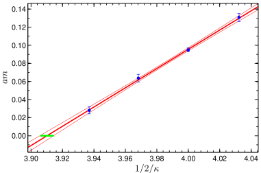
Figure 3: The PCAC quark mass from simulations at $\beta=7.2$ on $8^{3}\!\times\!12$ lattices. The additive mass shift is only $am_{{\rm add}}=0.090(4)$.

The remaining results quoted in this section are obtained from simulating a $12^{3}\times 24$ lattice at $\beta=7.2$ and $\kappa=0.1266$. We have accumulated 500 trajectories after thermalization and measured eigenvalues of $D$ and $\gamma_{5}D$, n-HYP smeared Wilson loops, as well as pseudoscalar correlators every 5 trajectories.

The three most expensive parts of the update are the calculation of the fermionic force (including inversions), the gauge force and the n-HYP blocking (including the n-HYP force term). Of the total CPU time in these runs they consumed 75%, 13% and 11%, respectively. Thus, even with inexpensive fermion formulations such as Wilson the computational overhead of the n-HYP blocking is negligible. One should also note that the inversions of the Dirac operator are expected to be significantly cheaper than in a comparable physical situation with thin link clover fermions if the latter is possible at all.

A few remarks on the details of our simulation are in place: Each trajectory was split in 25 steps using a Sexton-Weingarten integrator and the same integrator on a finer time scale was also used for the gauge force. This resulted in an acceptance rate of 0.879(7). On 32 nodes of a Myrinet cluster with 2GHz Xeon processors, one unit length trajectory took about 17 minutes to complete.

From fits to the static quark potential Hasenfratz et al. (2002b) we extract the Sommer scale Sommer (1994) $r_{0}/a=3.903(25)$ and the string tension $a\sqrt{\sigma}=0.2897(26)$. The bare current quark mass $am=0.0451(9)$ is in good agreement with the small volume data shown in Fig. 3, indicating small cutoff effects. Assuming $r_{0}=0.5\,$fm we obtain a lattice spacing of $0.128(1)\,$fm and bare current quark mass of $69.4(1.5)\,$MeV. We find a ratio of pseudoscalar to vector meson mass of $0.57(3)$.

The behavior of the low-lying eigenmodes of the Dirac operator are of particular interest if one wants to determine the degree of chiral symmetry that is retained at finite lattice spacing. Also, the lowest eigenvalue of the Hermitian Dirac operator $\gamma_{5}D$ is important for algorithmic reasons as it determines the spectral gap and indicates the lowest bare quark mass potentially accessible at a given lattice spacing and volume Del Debbio et al. (2006).

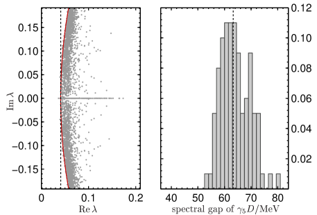
Figure 4: The infrared spectrum of the n-HYP Wilson clover Dirac operator (left panel), and the spectral gap as determined from the lowest eigenmode of the Hermitian $\gamma_{5}D$ Dirac operator on the same configurations (right panel). The dashed line in both plots indicates the median of the spectral gap distribution. Data are from 100 $12^{3}\times 24$ configurations with lattice spacing $a\approx 0.13\,$fm and bare quark mass $m\approx 69\,$MeV.

The left panel of Fig 4 shows the infrared spectrum (lowest 40 eigenmodes) of the n-HYP Dirac clover operator from 100 configurations. The complex spectrum has a rather well defined left boundary that follows a circle with only a few real modes violating that bound. This indicates that even at this coarse lattice spacing much smaller quark masses can be reached without encountering exceptional configurations. A similar plot is published in Ref. Lang et al. (2006) showing the eigenmodes of the chirally improved CI Dirac operator in two flavor dynamical simulations at similar lattice spacing and volume, though about 50% lighter quark masses. The spectrum in Fig. 4 compares well with that plot, showing similar widening of the Ginsparg–Wilson circle for the two actions.

A more direct measure of the accessible mass range is the spectral gap, i.e. the distribution of the smallest magnitude eigenvalue of the Hermitian Dirac operator $\gamma_{5}D$ Del Debbio et al. (2006, 2007). This distribution is plotted on the right panel of Fig. 4 with the median $\bar{\mu}=63.3(4)\,$ MeV marked by a dotted line. The ratio of the median and the PCAC quark mass is indicative of the renormalization factor $Z_{A}/(Z_{m}Z_{P})$ Capitani et al. (2006); Del Debbio et al. (2006) and the value we obtain, 0.91, signals small perturbative corrections.

To facilitate comparison with similar distributions in Ref. Del Debbio et al. (2006) the data is plotted with the same bin size, $\Delta\mu=1.5\,$MeV. The width of the distribution, defined as half the width of the shortest interval that contains 68.3% of the data, is $\sigma=5.5(6)\,$MeV. Since the distribution in Fig. 4 is quite asymmetric, it is more physical to define the width as the interval to the left of the median that contains 68.3% of the data. This modified definition gives $\sigma=4.6(6)\,$MeV. One expects that simulations at quark masses of about $3\sigma$ are safe, which corresponds to $\simeq 15\,$MeV at this volume and lattice spacing. In Ref. Del Debbio et al. (2006) it was found that, at least for unimproved thin link Wilson fermions Del Debbio et al. (2007), the width of the spectral gap scales inversely with the square root of the volume, $\sigma\sqrt{V}\approx 1$. Assuming the same scaling law in our case we find $\sigma\sqrt{V}\approx 0.61-0.73$, depending on the definition of the width. The decrease signals the improved chiral properties of the smeared Dirac operator. The median $\bar{\mu}$ of the lowest mode of the Hermitian operator is also indicated in the complex Dirac spectrum, where it is tangent to the circle that bounds the spectrum.

V Conclusions

We have successfully implemented and tested a gauge link smearing scheme that inherits the good properties of HYP smearing (locality and removal of dislocations) while still being suitable for MD based algorithms. This is achieved by replacing the projection steps in the original HYP construction by normalizations to the corresponding unitary group, thus allowing the calculation of the molecular dynamics force for fermions coupled to the smeared links. We have tested the n-HYP smearing with overlap fermions where we found that they can be simulated as effectively as 3 level stout smeared fermions and about twice as fast as 2-level stout smeared ones. We have also implemented the smearing with Wilson -clover fermions. Our preliminary tests indicate that light quarks, even as low as 15 MeV, can be simulated at $a\sim 0.13\,$fm lattices and volumes $aL\gtrsim 1.6$ fm. In addition, the smoothness of the smeared links speed up the inversion of the Dirac operator.

We have reported only preliminary results here. The volume, quark mass, and lattice spacing dependence of Wilson clover simulations with n-HYP links will be tested in the future.

VI Acknowledgment

At various stages of this project we have benefited from discussions with T. DeGrand, F. Niedermayer and T. Kovács. We thank the computer center of DESY at Zeuthen for providing us with essential resources and support. This research was partially supported by the US Dept. of Energy.

References

- Hasenfratz et al. (2002a) P. Hasenfratz, S. Hauswirth, K. Holland, T. Jorg, and F. Niedermayer, Nucl. Phys. Proc. Suppl. 106, 799 (2002a), eprint hep-lat/0109004.
- Neuberger (1998) H. Neuberger, Phys. Lett. B417, 141 (1998), eprint hep-lat/9707022.
- Orginos et al. (1999) K. Orginos, D. Toussaint, and R. L. Sugar (MILC), Phys. Rev. D60, 054503 (1999), eprint hep-lat/9903032.
- Hasenfratz and Knechtli (2001) A. Hasenfratz and F. Knechtli, Phys. Rev. D64, 034504 (2001), eprint hep-lat/0103029.
- Del Debbio et al. (2006) L. Del Debbio, L. Giusti, M. Lüscher, R. Petronzio, and N. Tantalo, JHEP 02, 011 (2006), eprint hep-lat/0512021.
- DeGrand et al. (1999) T. A. DeGrand, A. Hasenfratz, and T. G. Kovacs, Nucl. Phys. B547, 259 (1999), eprint hep-lat/9810061.
- DeGrand and Schaefer (2005a) T. DeGrand and S. Schaefer, Phys. Rev. D71, 034507 (2005a), eprint hep-lat/0412005.
- DeGrand and Schaefer (2005b) T. A. DeGrand and S. Schaefer, Phys. Rev. D72, 054503 (2005b), eprint hep-lat/0506021.
- DeGrand et al. (2003) T. DeGrand, A. Hasenfratz, and T. G. Kovacs, Phys. Rev. D67, 054501 (2003), eprint hep-lat/0211006.
- Albanese et al. (1987) M. Albanese et al. (APE), Phys. Lett. B192, 163 (1987).
- Morningstar and Peardon (2004) C. Morningstar and M. J. Peardon, Phys. Rev. D69, 054501 (2004), eprint hep-lat/0311018.
- Capitani et al. (2006) S. Capitani, S. Dürr, and C. Hoelbling, JHEP 11, 028 (2006), eprint hep-lat/0607006.
- Liang et al. (1993) Y. Liang, K. F. Liu, B. A. Li, S. J. Dong, and K. Ishikawa, Phys. Lett. B307, 375 (1993), eprint hep-lat/9304011.
- Zanotti et al. (2002) J. M. Zanotti et al. (CSSM Lattice), Phys. Rev. D65, 074507 (2002), eprint hep-lat/0110216.
- DeGrand and Liu (2005) T. A. DeGrand and Z.-f. Liu, Phys. Rev. D72, 054508 (2005), eprint hep-lat/0507017.
- DeGrand et al. (2006a) T. DeGrand, R. Hoffmann, S. Schaefer, and Z. Liu, Phys. Rev. D74, 054501 (2006a), eprint hep-th/0605147.
- DeGrand and Schaefer (2006) T. DeGrand and S. Schaefer, JHEP 07, 020 (2006), eprint hep-lat/0604015.
- DeGrand et al. (2006b) T. DeGrand, Z. Liu, and S. Schaefer, Phys. Rev. D74, 094504 (2006b), eprint hep-lat/0608019.
- Egri et al. (2006) G. I. Egri, Z. Fodor, S. D. Katz, and K. K. Szabo, JHEP 01, 049 (2006), eprint hep-lat/0510117.
- DeGrand (2001) T. A. DeGrand (MILC), Phys. Rev. D63, 034503 (2001), eprint hep-lat/0007046.
- Hasenfratz et al. (2002b) A. Hasenfratz, R. Hoffmann, and F. Knechtli, Nucl. Phys. Proc. Suppl. 106, 418 (2002b), eprint hep-lat/0110168.
- Sommer (1994) R. Sommer, Nucl. Phys. B411, 839 (1994), eprint hep-lat/9310022.
- Lang et al. (2006) C. B. Lang, P. Majumdar, and W. Ortner, Phys. Rev. D73, 034507 (2006), eprint hep-lat/0512014.
- Del Debbio et al. (2007) L. Del Debbio, L. Giusti, M. Lüscher, R. Petronzio, and N. Tantalo (2007), eprint hep-lat/0701009.